Abstract— In this paper, we propose a generalized fuzzy inference
system (GFIS) in noise image processing. The GFIS is a multi-layer neuro-fuzzy structure which combines both Mamdani model and TS fuzzy model to form a hybrid fuzzy system. The GFIS can not only preserve the interpretability property of the Mamdani model but also keep the robust local stability criteria of the TS model. Simulation results indicate that the proposed model shows a high-quality restoration of filtered images for the noise model than those using median filters or wiener filters, in terms of peak signal-to-noise ratio (PSNR).
Index Terms—Generalized Fuzzy Inference System, Mamdani
model, TS model, PSNR
I. INTRODUCTION
The image corrupted by different kinds of noises is a frequently encountered problem in image acquisition and transmission [1]. The noise comes from noisy sensors or channel transmission errors. Several kinds of noises are discussed here. The impulse noise (or salt and pepper noise) is caused by sharp, sudden disturbances in the image signal; its appearance is randomly scattered white or black (or both) pixels over the image. Gaussian noise is an idealized form of white noise, which is caused by random fluctuations in the signal. Speckle noise (or more simply just speckle) can be modeled by random values multiplied by pixel values, hence it is also called multiplicative noise. If the image signal is subject to a periodic, rather than a random disturbance, we might obtain an image corrupted by periodic noise. Usually, periodic noise requires the use of frequency domain filtering. This is because whereas the other forms of noise can be modeled as local degradations, periodic noise is a global effect. However, impulse noise, gaussian noise and speckle noise can all be cleaned by using spatial filtering techniques, such as Order Statistic Filter (OSF). Order statistic filters have been applied to image processing problems [2]. Given N observations X1,
X2,…,XN of a random variable X, the order statistics are
obtained by sorting the {X(i)} in ascending order. This produces {X(i)} satisfying X(1)≤X(2)≤…≤X(N). The {X(i)} are the order statistics of the N observations. The order statistic filter is an estimator F(X1,X2,…,XN) of the mean of X which uses a linear
combination of order statistics
(1) Some common filters which fit the order statistic filter framework are the linear average filter, the median filter, and trimmed mean filer. Among them, the median filter sorts the surrounding pixels values in the window to an orderly set and replaces the center pixel within the define window with the middle value in the set. That means the coefficients αi’s in are
defined as
(2) In (2), N is an odd number. The median filtering is a non-linear filtering technique that works best with impulse noise whilst retaining sharp edges in the image. Although the median filter can achieve reasonably good performance for low corrupted images, it will not work efficiently when the noise rate is too high. Another disadvantage of the median filter is the extra computation time needed to sort the intensity value of each set. Many other improved algorithms, such as weighted [3] or center-weighted median filter [4], have been proposed to improve their performances.
Recently, application of fuzzy techniques in image noise reduction processing is a promising research field [5]. Fuzzy techniques have already been applied in several domains of image processing, e.g. filtering, interpolation, and morphology, and have numerous practical applications in industrial and medical image processing. These fuzzy filters, including FIRE-filter [6], the weighted fuzzy mean filter [7], and the iterative fuzzy control based filter [8], are able to outperform rank-order filter schemes (such as the median filter). Nevertheless, most fuzzy techniques are not specifically designed for gaussian(-like) noise or do not produce convincing results when applied to handle this type of noise. In this paper we proposed a generalized fuzzy inference mode, which is a hybridizations of the Mamdani and TS models. The GFIS can be characterized by the neuro-fuzzy spectrum, in light of linguistic transparency and input-output mapping accuracy.
In section II, the concepts of fuzzy basis function (FBF) are introduced. The fuzzy basis functions expansion can be regarded as a general form of fuzzy system. Two famous fuzzy inference modes are also introduced. The similarities between them are also discussed to provide the foundation of the GFIS. In section III, the GFIS and its representation in neuro-fuzzy
Image Denoising Using Adaptive Neuro-Fuzzy
System
Nguyen Minh Thanh
and Mu-Song Chen
1, ( 1) / 2
0, otherwise
i
i N
α = = +
1 2 1 (1) 2 (2) ( )
( , , , N) N N
F X X X =α X +α X + +α X
IAENG International Journal of Applied Mathematics, 36:1, IJAM_36_1_11
______________________________________________________________________________________
architectures are demonstrated. Section IV shows the simulation results and our conclusions are given in the last section.
II. FUZZY BASIS FUNCTIONS AND FUZZY INFERENCE MODELS
Fuzzy systems with singleton fuzzification, product as the fuzzy conjunction operator, addition for fuzzy rule aggregation, and center of average defuzzification, can be expressed as a linear combination of K fuzzy basis functions (FBFs) [9] in the following
(3) where
y
k is the center of gravity of the output fuzzy set andφk(x) are called fuzzy basis functions and are given by
(4)
µkj(xj) denotes the membership function of input xj belonging to
the kth rule, µkj : R→ [0,1]. Note that (4) is not well-defined if
1 1 ( ) 0
K n
mj j
m= j=µ x =
∑ ∏
for some x, which could happen if the input space is not wholly covered by fuzzy rule patches. However, there are several easy fixes for this problem. For example, we can either force the output to some constant when the denominator is zero, or add a fuzzy rule so that the denominator is always greater than zero for all x.On the basis of the stone-weierstrass theorem [10], the universal approximation theorem was demonstrated that an FBF network can perform approximation of continuous function to arbitrary accuracy. Consequently, the expression of fuzzy models by fuzzy basis functions makes the models more easily in solving model’s parameters. The universal function approximation property gives a strong mathematical ground when applying fuzzy system in critical applications, ranging from control, to time series prediction, to patterns recognition as well as image processing.
In this paper, we study the fuzzy system based on a multiple-input/multiple-output (MIMO) of the FBF network. Specially, if there are n-input, K fuzzy rules and m-output, the
kth rule’s activation can be written as
(5) In fact, rk is the degree (or the firing strength) the input x
matches rule computed by the T-norm or product operator. The membership function can have different shapes. For an extensive overview of other membership functions, the reader is referred to [11]. In this study, we choose Gaussian function as the membership function
(6) The output value of the ith output is
(7) for i = 1,2,…,m and yik is the center of gravity of the kth aggregated output fuzzy membership function associated with the output yi.
In general fuzzy systems represented by (7) can be broadly categorized into two families, depending on the THEN-part of fuzzy rules and the way to combine fuzzy rules. The first one includes linguistic models based on collections of IF–THEN rules, whose antecedents and consequents utilize fuzzy sets. The Mamdani model [12] falls in this group. The Mamdani model uses fuzzy reasoning and the system behavior can be described in natural ways. A Mamdani model is presented as a collection of fuzzy rules in the following form
(8) where x = [x1,x2,…,xn]T∈Rn and scalar y are the input and
output linguistic vectors, respectively. 1k, 2k, , k n A A A and Bk
are the corresponding fuzzy sets for x and y in rule k. It can be found from (8) that rule k maps a fuzzy region in the input space to fuzzy regions in the output space by inference mechanisms, such as max-min or max-product inferences. In Mamdani model, by using max-product inference mechanism and center of average defuzzification, the output yi can be expressed as
(9) We can replace the integral in (9) with small discrete sums indexed only by the number of fuzzy sets that quantize the fuzzy variables. This eliminates both the need to approximate the centroid and its computational burden. Therefore,
(10) where rk is the same as in (5), vk is the volume of the output
fuzzy set Bkand bk is the corresponding centroid of Bk' which is
the scaled output set of Bk. In the applications of Mamdani
model, such classification or approximation of static functions, the linguistic rules usually can be understandable to the user who does not have to be an expert in the considered problem domain. Without aiming at its accuracy, fuzzy systems constructed by Mamdani models are comprehensible and interpretable
.
This is a very important property, since it allows the transformation of numerical data or vague knowledge into fuzzy rules.The second category, based on Takagi-Sugeno (TS) model systems [13], uses a rule structure that has fuzzy antecedent and functional consequent parts. For TS model, the fuzzy knowledge is represented as
(11)
1 1 2 2
Rule : If is and is and is then is
k k k
n n
k
k x A x A x A
y B
1 1 2 2
Rule : If is and is and is then is ( )
k k k
n n
k
k x A x A x A
y f x
1 ( )
K k k k
y=
∑
= yφ
x1 1 1 ( ) ( ) ( ) n kj j j
k K n
kj j k j x x
µ
φ
µ
= = = =∏
∑ ∏
x1 ( )
n
k j kj j
r =
∏
=µ
x2 1
( ) exp 2 j kj kj j kj x c x µ σ − = − 1 1 1 ( )
K k K
i k K ik k ik k
k k
r
y y y
r
φ
= = = =∑
=∑
∑
x ( ) ( ) k y i k yyB y dy y
B y dy =
∫
∫
1 1
K k k k k
i K
k k k
Depending on the form of fk(x), a singleton or a linear
combination of input vector, equation (11) can describe either a zero-order or first-order TS model. For a first-order TS model,
fk(x) can be a linear function of x, i,e.,
(12) In(12) X is the augmented vector of x, X = [1,x1,x 2,…,xn]T and
pk = [pk0,pk1,…,pkn]T is the coefficient vector. The dot in (12)
denotes the inner product of two vectors. In the first-order TS model, the rule’s output y determines a local input-output relation by means of the real-valued coefficient vector pk and
therefore the corresponding hyper-planes characterizing the local structure of the function to be approximated. The feature of locality of the TS model allows us to represent even quite complicate input-output relationships through a collection of local models. For any input x, the system output yi is computed
by centroid defuzzification
(13) Because the outputs are calculated as a weighted average of the individual outputs, a sort of smooth transition of the individual models should be guaranteed. Therefore, TS models are capable of approximating any continuous real-valued function on a compact set to any degree of accuracy [14]. The obtained rule set from the first-order TS model can be used to provide system output values for any given input values through an interpolation of all the relevant individual rules. Such models are capable of representing both qualitative and quantitative information and allow relatively easier application of powerful learning techniques for their identification from data. This type of knowledge representation, however, does not allow the output variables to be described in linguistic terms and the parameter optimization is carried out iteratively using a nonlinear optimization method. There is a tradeoff between readability and precision. If one is interested in a more precise solution, then one is usually not so bothered about its linguistic interpretability. Sugeno-type systems are more suitable in such cases. Otherwise, the choice is for Mamdani-type systems. Therefore, the combination of both the Mamdani and TS model as neuro-fuzzy models appear as an attempt to merge the advantages of both systems in terms of transparency with the advantages of learning capabilities.
From (8) and (11), the Mamdani and TS models are different in THEN-part only, therefore both models can be expressed in a more compact form as
(14) where Fk can be either Bk for the Mamdani model or fk for the
TS model. In this way, the fuzzy system representation in (14) is consistent with that of the fuzzy basis functions expansion in (7) and the Mamdani model is expressed as
(15)
while the TS model is
(16) It is very obvious that (15) and (16) share the similarity by using a linear combination of FBFs. With the conditions of v1 =
v2 =…= vK, where the Mamdani model owns the same size of
output membership functions, and fk(x) = bk, where the TS
model is zero-order, (15) and (16) become equivalent. Consequently, the general form of (15) and (16) is
(17) Equation (17) is the hybridizations of both models and a generalized fuzzy inference model (GFIS), which is an integration of the merits of Mamdani and TS models, an be designed to build a more readable model while maintains its precision.
In the next section, the GFIS model is presented by the neuro -fuzzy network architecture [15][16]. The neuro-fuzzy network, which is an integration of the merits of neural and fuzzy approaches, enables one to build more intelligent decision-making systems. This incorporates the generic advantages of artificial neural networks like massive parallelism, robustness, and learning in data-rich environments into the system. The modeling of imprecise and qualitative knowledge as well as the transmission of uncertainty are possible through the use of fuzzy logic. Besides these generic advantages, the neuro–fuzzy approach also provides the corresponding application specific merits. Specially, the GFIS is designed for multiple outputs in each rule such that the model can be extended to more real-world applications. Besides, for the applications of pattern recognition, the obtained model can be considered as an extension of the quadratic Bayes classifier that utilizes mixture of models for estimating the class conditional densities.
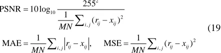
III. GENERALIZED FUZZY INFERENCE SYSTEM,GFIS The proposed GFIS is assumed to have n inputs, K rules, and
m outputs in each rule. Fig. 1 shows the GFIS with two inputs, four rules, and three outputs. Each rule in the GFIS is written as
(18) In (18), the output membership function Bkj(.) is characterized
by two pavements, vk and fkj(x). vk, which is common to rule k,
represents the area of Bkj(.) and fkj(x) is the centroid of Bkj(.).
The essential feature of (18), when compared with (8) or (11), is the output representation of the consequent parts. The GFIS can not only preserve the interpretable capability of the Mamdani model but also maintain the accuracy of the TS model.
To optimize the system performance, a two-phased hybrid parameter learning algorithm is applied with a given network structure. In hybrid learning, each iteration is composed of a
0 1 1
( )
k k k k kn n
f x =p Xi = p +p x + +p x
1 1 ( ) K k k k i K k k r f y r = = =
∑
∑
x1 1 2 2
Rule : If is and is and is then is
k k k
n n
k
k x A x A x A
y F
1 1
( )
K k
i k K k
k k r y f r = = =
∑
∑
x 1 1K k k
i k K k
k k k r v y b r v = = =
∑
∑
1 1 ( )K k k
i k K k
k k r v y f r = = =
∑
∑
x1 1 2 2
1 1 1
Rule : If is and is and is then ( , ( )) ...and ( , ( ))
k k k
n n
k k k m km k km
k x A x A x A
forward pass and a backward one. In the forward pass, after the input vector is presented, we calculate the node outputs in the network layers and on the basis of this the linear parameters are adjusted using pseudo inverse based on recursive least-squared technique. After the linear parameters are identified we can compute the error for training data pairs. In the backward pass the error signals propagate from the output end toward the input nodes; the gradient vector is calculated and the nonlinear parameters updated by steepest descent method. The learning step of the nonlinear parameters update is adjusted using adaptive approach. This process is repeated many times until the system converges or error is below some predefined threshold. Detail descriptions of the parameter-tuning method can be found in [19].
IV. SIMULATION RESULTS
The proposed model is tested for removing salt-and-pepper impulse noise and Gaussian noise. The noisy image is divided by several pxp block. Each image block is fed into the GFIS model. The inferred output from the GFIS is compared with the noise-free image block. Fig. 2 shows the schematic diagram for noisy image processing. The proposed filter is applied to grayscale test images, after adding either Gaussian noise or salt-and-pepper noise of different levels. Such a procedure allows us to compare and evaluate the filtered images against the original images. In the case of salt and pepper, images will be corrupted by “salt” (with value 255) and “pepper” (with value 0) with equal probability. A wide range of salt-and-pepper noise levels varied from 10 % to 90 % with increments of 5 % will be tested. Also the additive Gaussian white noise is zero mean with varied variance from 0.1 to 0.9. Restoration performances are quantitatively measured by the peak signal-to-noise ratio (PSNR) and the mean absolute error (MAE), and mean squared error (MSE) [18]
(19)
where NxM is the number of processed pixels and rij and xij
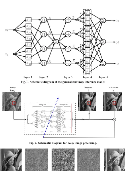
denote the pixel values of the restored image and the original image, respectively. For comparison purpose, the 3x3 median filter and the 3x3 wiener filter are tested to compare with our proposed GFIS. In the first test, a 8-bit grayscale image of Lena
[image:4.595.60.281.500.553.2]is corrupted by salt-and-pepper noises. We summarize the restored images of median filter, wiener filter, and the GFIS in Fig. 3. Among the restorations, our proposed GFIS gives the best performance in terms of noise suppression and detail preservation. The median filter and the wiener filter can achieve reasonably good performance for low corrupted images, but they will not work efficiently when the noise level is above 50%. From visual differences, salt-and-pepper noise with noise ratio as high as 90% can be cleaned quite efficiently. In addition, the GFIS requires only 2 rules and 236 free parameters to be tuned. The compact structure makes the model
learn very fast.
The second simulation is conducted by adding zero mean Gaussian noise in tests image with different variance. The variance starts from 0.1 to 0.9 with increments of 0.1. Fig. 4 shows plots of PSNR, MAE, and MSE versus variance of Gaussian noise. From the plots, we have found that all the methods have similar performance when the noise level is low. This is because the median and wiener filters focus on the noise detection. However, when the noise level increases, noise patches will be formed and they may be considered as noise free pixels. This causes difficulties in the noise detection and removal and the results of filtered images are not recognizable. On the other hand, our denoising method achieves a high PSNR and low MAE even when the noise level is high. This is mainly based on the accurate noise detection by the adaptive neuro-fuzzy model. Experimental results show that the GFIS impressively outperforms other techniques.
V. CONCLUSION
This paper proposed an adaptive neuro-fuzzy approach for additive noise reduction. The main feature of the GFIS is the hybridizations of the Mamdani and TS models. Experimental results are obtained to show the feasibility and robustness of the proposed approach. These results are also compared to other filters by numerical measures and visual inspection. In the near future, we will extend GFIS to process color images. Moreover, the uniform distribution impulsive noise model will be further studied.
ACKNOWLEDGMENT
This research was supported by the National Science Council under contract number NSC94-2213-E-212-036.
REFERENCES
[1] R. C. Gonzalez and R. E. Woods, Digital Image Processing, 2nd ed. Englewood Cliffs, NJ: Prentice-Hall, 2001. [2] A. C. Bovik, T. S. Huang, and D. C. Munson. A
generalization of median filtering using linear combinations of order statistics. IEEE Transactions on
Acoustics, Speech, and Signal Processing,
31(6):1342-1349, December 1983.
[3] D. Brownrigg, “The weighted median filter,” Commun. Assoc. Comput., pp. 807–818, Mar. 1984.
[4] S. J. Ko and S. J. Lee, “Center weighted median filters and their applications to image enhancement,” IEEE Trans. Circuits Syst., vol. 15, no. 9, pp. 984–993, Sep. 1991. [5] E. Kerre and M. Nachtegael, Eds., Fuzzy Techniques in
Image Processing. New York: Springer-Verlag, 2000, vol. 52, Studies in Fuzziness and Soft Computing.
[6] F. Russo and G. Ramponi, “A fuzzy operator for the enhancement of blurred and noisy images,” IEEE Trans. Image Processing, vol. 4, pp. 1169–1174, Aug. 1995. [7] C.-S. Lee, Y.-H. Kuo, and P.-T. Yu, “Weighted fuzzy
mean filters for image processing,” Fuzzy Sets Syst., no. 89, pp. 157–180, 1997.
2 10
2 ,
2
, ,
255
PSNR 10 log
1
( )
1 1
MAE , MSE ( )
ij ij i j
ij ij ij ij
i j i j
r x MN
r x r x
MN MN
=
−
= − = −
∑
[8] F. Farbiz and M. B. Menhaj, Fuzzy Techniques in Image Processing. New York: Springer-Verlag, 2000, vol. 52, Studies in Fuzziness and Soft Computing, ch. A fuzzy logic control based approach for image filtering, pp. 194–221.
[9] Kim, H.M., and Mendel, J.M.. ”Fuzzy basis functions: Comparisons with other basis functions.” IEEE Trans. on Fuzzy Systems, 3, 1995, pp. 158–168.
[10]Rudin, W. Principles of Mathematical Analysis. McGraw-Hill, Inc., 1960.
[11]Yager, R. and Filev, D., “Approximate clustering via the mountain method,” IEEE Transactions on Systems, Man and Cybernetics. 24(8): 1279-1284, 1994.
[12]E. H. Mamdani and S. Assilian, “An experiment in linguistic synthesis with a fuzzy logic controller,” International Journal of Man-Machine Studies, 7(1):1-13, 1975.
[13]T. Takagi and M. Sugeno, “Fuzzy identification of systems and its applications to modeling and control,” IEEE Trans. Syst., Man, Cybern., vol. 15, pp. 116–132, Jan. 1985. [14]J. J. Buckley and T. Feuring, Fuzzy and Neural:
Interactions and Applications, ser. Studies in Fuzziness and Soft Computing. Heidelberg, Germany: Physica-Verlag, 1999.
[15]C. T. Lin and C. S. George Lee, Neural Fuzzy Systems--A Neuro-Fuzzy Synergism to Intelligent Systems. Englewood Cliffs, NJ:Prentice-Hall, 1996.
[16]J. S. R. Jang, C. T. Sun, and E. Mizutani, Neuro-Fuzzy and Soft Computing. Englewood Cliffs, NJ: Prentice-Hall, 1997.
[17]A. Papoulis, Probability, Random Variables, and Stochastic Processes, McGraw Hill, Inc., 1984.
[18]A. Bovik, Handbook of Image and Video Processing. New York: Academic, 2000.
[19]Nguyen Minh Thanh, “Structure learning and Parameter Learning for neuro-fuzzy model”, Ms Thesis, June, 2006.
Fig. 1. Schematic diagram of the generalized fuzzy inference model.
Fig. 2. Schematic diagram for noisy image processing.
Fig. 3. Restoration results. (a). Original image. (b). Corrupted Lena image with 90% salt-and-pepper noise (53.7 dB). (c). median filer (54.45 dB). (d). wiener filer (59.35 dB). (e). GFIS (66.06 dB).
(a) (b) (c) (d) (e)
Noisy imag
Restore d
[image:6.595.94.497.117.361.2]Fig. 4. Results in PSNR, MAE, and MSE for the Clown image at various variance levels for median filter, wiener filter, and GFIS.
10 20 30 40 50 60 70 80 90 50
55 60 65 70
var
PS
NR
(
d
B
)
clown, Gau noise, mean PSNR = 65.8759
10 20 30 40 50 60 70 80 90 0
0.1 0.2 0.3 0.4
var
MA
E
clown, Gau noise, mean MAE = 0.10067
10 20 30 40 50 60 70 80 90 0
0.05 0.1 0.15 0.2 0.25
var
MS
E
clown, Gau noise, mean MSE = 0.017823