Asymmetric Liquidity Risk Premia in Intraday High
Frequency Trading
Jun Qi
∗Wing Lon Ng
†Abstract—The traditional Value at Risk (VaR) is a very popular tool for measuring market risk, but
it does not incorporate liquidity risk. This paper
proposes an extended VaR model to integrate liquid-ity risk in intraday trading strategies when analyzing high frequency order book data. We estimate the one step ahead liquidity adjusted intraday VaR (LAIVaR) for both bid and ask positions, considering several threshold trading sizes. We also quantify the liquid-ity risk premium by comparing our result with the standard VaR approach, applying the approach in 3 UK bank stocks. The liquidity risk premia of differ-ent volumes for the Northern Rock stock are larger on the bid side in 5 minutes and 10 minutes trading intervals. In contrast, in the case for the Royal Bank of Scotland, the liquidity risk premium on the ask side is larger than on the bid side when the volume is high. For HSBC, the liquidity risk premium is roughly the same on both sides.
Keywords: Liquidity adjusted intraday VaR, liquidity risk premium, asymmetric market behaviour.
1
Introduction
The growth of the risk management industry can be traced directly to the increased volatility of financial mar-ket since the early 1970s. Liquidity risk is a key factor of the cause of many serious market crises. The infa-mous disaster from the Long Term Capital Management (LTCM) in late 1998, Russian financial crisis in 1998 and the collapse of credit market in 2008 evidence the dangers of ignoring the effects of liquidity. In September 2007,the British retail bank Northern Rock could not refinance it-self in the credit market and faced bankruptcy due to the lack of liquidity. These big lessons teach us that the liquidity plays a very important role in financial mar-kets, in particular when it comes to trading. Therefore, a good risk measurement has to take liquidity risk in to ac-count. However, the definition of liquidity is ambiguous and has many different interpretations. “A liquid mar-ket is a marmar-ket in which a bid-ask price is always quoted, its spread is small enough and small trades can be
im-∗Corresponding author. E-mail:[email protected]
†Wing Lon Ng is grateful to the German Research Foundation
(DFG) for financial support through research grant 531283. Both authors would like to thank seminar participants at the University of Essex for their helpful comments and Jian Jiang who provided the order book data.
mediately executed with minimal effect on price (Black (1971))”.
A concept that is even more difficult to predict and mea-sure isliquidity risk. In a real “friction market”, investors hardly get the mid-price that is used in many risk applica-tions and a more rigorous approach of risk management is needed. Bangia, Diebold, Schuermann, and Stroughair (1999) argue that the liquidity risk is an impor-tant component in order to capture the overall risk. Lawrence and Robinson (1997) stress that the failure to consider liquidity may lead to an underestimation of the VaR by 30%.
Although more and more market practitioners have recognized that liquidity risk is a very serious concern for firms, plenty studies have separately analyzed the VaR and liquidity. Only a few studies incorporate liquidity into VaR, not to speak of VaR at intra-day level (see, for example, Beltratti and Morana (1999), Dionne, Duchesne, and Pacurar (2006) or Colletaz, Hurlin, and Tokpavi (2007)). The literature include only a few former studies where researchers have incorporated liquidity risk with conventional VaR. In general, there are two different methods: the first one is the stochastic horizon method. Lawrence and Robinson (1997) determine the holding period of VaR accord-ing to the size of position and the characteristics of liquidity market. The second method models market price changes induced by the selling the underly-ing asset within a fixed time horizon. For example, Glosten, Jagannathan, and Runkle (1997) use this method to derive the optimal strategy of liquidation that maximize the value over a pre-specified period. Therefore, they consider the impact of the size of the position and the period of execution on the value under liquidation of the position. Bertsimas and Lo (1998) use a similar method to determine the dynamic optimal strategy for minimizing the cost of execution.
un-der real market conditions, especially in intraday trading, as execution is not always guaranteed, i.e. the conven-tional VaR models do not capture the liquidity risk that traders and investors are exposed to. This paper there-fore attempts to measure additional risk due to liquidity in the VaR using intraday data and extends the existing literature in the following way: We consider the endoge-nous liquidity risk, taking into account the volume effect to model the liquidity adjusted intraday VaR (LAIVaR), which measured on the basis of the size of investors’ po-sitions.
Secondly, the result shows that there is an asymmetry in up and down movement in the equity market. Downward movements typically have a higher magnitude than up-ward movements. Xiangli L (2008) prove the upside risk is important by studying upside VaR and extreme up-side risk spillover in Chinese copper futures market and spot market. Our paper investigates both upside and downside VaR process. In particular, we are interested in differentiating between both bid and ask sides since different market sides have to face different price move-ments as well. We estimate the one step ahead LAIVaR of both market sides in order to quantify their real risk position.
The outline of the paper is as follows. Section 2 provides a literature review. Section 3 describes the methodology and Section 4 presents the data and the empirical results. Section 5 concludes.
2
Literature Review
2.1
Liquidity and Liquidity Risk
Liquidity plays a very important role in the financial mar-ket. However, the definition of liquidity is ambiguous and has several versions. Generally speaking, the liquidity is a ability for participants to execute large trades rapidly at with a small impact on prices (CGFS (2000)).
Figure 1: The relationship between liquid and illiquid position of VaR and holding period (Source Dowd (1998)
Market liquidity risk can be summarized as the risk aris-ing from the higher cost and difficulty to execute the trade
which is caused by illiquidity market. According to Dowd (1998) “a market can be very liquid most of the time, but lose its liquidity in a major crisis”. In general, we could differentiate the liquidity risk between normal liquidity risk and crisis liquidity risk. During the crisis period, the liquidity risk should be taken more serious in to account because market lose its liquidity. Dowd (1998) also point out the relationship between the liquid position of VaR and the holding period (see Figure 1). In a highly liquid position the investors can settle the position quickly to get the market price without any significant liquidation cost. But in a illiquid position, one must pay liquidity cost to close his position. The longer the investor wait, the lower of liquidity cost. Moreover, during the waiting period, the asset price can change in a worse way.
Bangia, Diebold, Schuermann, and Stroughair (1999) di-vide the liquidity risk into two components. Exogenous liquidity risk is influenced by the character of market. On the other hand, endogenous liquidity risk is specific af-fected by participant’s action and position. For example, the larger the trade size, the bigger the ask-bid spread, and the higher the endogenous liquidity risk will become. Figure 2 shows the relationship between the endogenous risk and the the investors’ position.
Figure 2: The effect of position size on liquidation value. Source: Bangia, Diebold, Schuermann, and Stroughair (1999)
2.2
Models of Liquidity Adjusted VaR
Conventional VaR models have an implied assumption which is that an asset can be traded at a fixed price within a fixed period of time. This assumption is not realistic un-der real market conditions. Obviously, the conventional VaR models do not capture the liquidity risk.
pe-riod of VaR according to the size of position and the char-acteristics of liquidity market. The authors use the sec-ond kind of method which is deriving the optimal strategy of liquidation that will maximize the value over a fixed time horizon. Glosten, Jagannathan, and Runkle (1997) therefore consider the impact of the size of the position and the period of execution on the value under liquidation of the position. Bertsimas and Lo (1998) use the similar method to derive the dynamic optimal strategy with the aim of minimizing the expected cost.
Bangia, Diebold, Schuermann, and Stroughair (1999) develop a liquidity adjusted VaR (LAVaR) model (named as the BDSS model after the name of the authors) which is a fundamental framework for integrating liquidity risk into the standard VaR. The BDSS model mainly focuses on exogenous liquidity risk which take the bid-ask spread into account. The LAVaR simply represents the sum of conventional VaR (computed by mid-price) and the liquidity risk adjusted part (computed by ask-bid spread).
LAV aR=M idt[(1−eµ−ασ) +
1 2(S+α
′σ)]˜ (1)
where M idt is the mid-price of the asset at time t, S =
(Ask−Bid)/M idis the the average relative spread,σ˜ is the volatility of relative spread and α′ is the quantle of the relative spread distribution.
However, the BDSS model has several drawbacks: Firstly, the model is based on the normal distribution which dif-fers from reality. Secondly, the method ignores the en-dogenous liquidity risk which is also important. Thirdly, the assumption of perfect correlation between liquidity risk and VaR would lead to an overestimation of the LAVaR. Erwan (2001) extends the BDSS model by us-ing the weighted average spread which incorporates the endogenous risk effect instead of the ask-bid spread. He also points out that for illiquid stocks, the endogenous liquidity risk represents half of the total market risk and must not be neglected.
Hisata and Yamai (2000) propose a framework for the quantification of the LAVaR model that considers the market impact induced by the trader’s own liquidation. They derive the optimal execution strategy according to level of market liquidity and the scale of the investor’s position. They choose the holding period as an endoge-nous variable and provide both a discrete time model and continuous time model for LAVaR measurement.
Further, Agnelidis and Benos (2006) investigate intraday LAVaR in Athens Stock Exchange and extend the model from Madhavan, Richardson, and Roomans (1997) by in-corporating trading volume and take both endogenous and exogenous liquidity risk into account. Their result also shows that the liquidity risk must not be neglected. Moreover, the LAVaR exhibits a U-shaped pattern
throughout the day. In contrast, Giot and Gramming (2006) introduce a GARCH model to derive the LAVaR in an automated auction market. Their empirical model is based on the BDSS framework and model the liquidity risk by calculating the weighted average bid price from the real order book data. They incorporate the endoge-nous risk impact by corresponding the trader’s position. Their result shows that liquidity in VaR accounts signifi-cantly and the liquidity risk exhibits an L-shape pattern throughout the day.
Agnelidis and Benos (2006) investigate intraday LAVaR in Athens Stock Exchange. They extend the model from Madhavan, Richardson, and Roomans (1997) by taking in to account trading volume and both endogenous and exogenous liquidity risk. Their result also shows that the liquidity risk must not be neglect. Moreover, the LAVaR exhibits a U-shaped pattern throughout the day.
As showed in Figure 3, the conventional VaR model like RiskMetrics (Morgan (1996)) measures the uncertainty of assets returns and do not include the liquidity risk. So a improved approach of modeling VaR should take the whole market risk into account.
Figure 3: Taxonomy of Market Risk and
the VaR Models (Source: Adapted from
Bangia, Diebold, Schuermann, and Stroughair (1999).)
2.3
Multivariate GARCH Models
Multivariate GARCH models were initially developed in the late 1980s. Basically the models study the mov-ing process both of variance and covariances which is different with univariate GARCH models. There are three important classes of multivariate models, namely (a) the VECH model, (b) the diagonal VECH model Bollerslev, Engle, and Wooldridge (1998) and (c) the BEKK model Engle and Kroner (1995).
The VECH model is proposed by
Bollerslev, Engle, and Wooldridge (1998) which is the original version of the multivariate GARCH model:
withεt|Ψt−1∼N(0, Ht), and
V ech(Ht) =C+ q
X
i=1
AiV ech(εt−iε0t−i)+ p
X
j=1
BjV ech(Ht−j)
(3) where Yt is an N ×1 vector which denotes the return
at time t, µt is the conditional mean of Yt, εt is the
in-novation vector, Ψt−1 is the set of information available
time t−1, C is a N(N + 1)/2×1 vector, Ai and Bj
areN(N+ 1)/2×N(N+ 1)/2matrices, andV ech(.) de-notes the column-stacking operator applied to the lower portion of anN×N symmetric matrix.
The number of parameters in VECH model equals:
2N(N+1)+N2(N+1)2(p+q)
4 . For example, if we assume N=2,
and the simple GARCH(1,1) model, then there are 21 pa-rameters need to be estimated; if N=3, then there are 78 parameters need to be estimated. Thus, the estimation of VECH model is very complex.
Therefore Bollerslev, Engle, and Wooldridge (1998) de-velop the diagonal VECH model in order to reduce the parameters to estimate in VECH model, which is written as:
hij,t=ωij+αijεi,t−1εj,t−1+bijhij,t−1 (4)
whereωij,αij andbij are parameters.
Later, Engle and Kroner (1995) present the BEKK model which imposes positive definiteness restrictions to ensure the H matrix being positive. The general format of con-ditional covariance matrix can be represented as:
Ht=CC0+ ΣKk=1Σqi=1Aikεt−iε0t−iA0ik
+ΣK
k=1Σpi=1BikHt−iBik0
(5)
where C is a lower triangular parameter matrix,Aikand BikareN×N matrices. As long asCis positive definite,
the conditional covariance matrix is also positive definite because the other terms in (4) are expressed in quadratic form.
For example, we assume K= 1and apply GARCH(1,1) model:
Ht=CC0+A11εt−1ε0t−1A011+B11Ht−1B110 (6)
In the bivariate case, the BEKK becomes
Ht=CC0+A
·
ε2
1t−1 ε1t−1ε2t−1
ε2t−1ε1t−1 ε22t−1
¸
A0
+B
·
h11t−1 h12t−1
h21t−1 h22t−1
¸
B0 (7)
where
A=
·
a11 a12
a21 a22
¸
B =
·
b11 b12
b21 b22
¸
.
The commonly method to estimate a multivariate GARCH model is conditional log likelihood function which has the following form:
L(θ) =−T N
2 ln2π− 1 2
T
X
t=1
(ln|Ht|+εtHt−1εt) (8)
where θ denotes the vector of all the unknown param-eters, and Ht = (σijt)N×N. Numerical maximization
yields the maximum likelihood estimates with asymptotic normal standard errors.
3
Methodology
Different positions face different risks. Developing the discussed models further, we estimate the liquidity ad-justed intraday VaR (LAIVaR) model for the bid side, which is for the investor who wants to buy, as well as for the ask side, which is for the investor who wants to sell. Researchers normally use daily data to analysis financial problems. Compared with the low frequency data, the shorter time horizon of high frequency data can present more detailed information about the market behavior. Letvi,tdenote the corresponding volumes of orders
queu-ing in the book at timetat positionsi= 1, ..., n. Similar to Giot (2005), we first define for both bid (B)and ask
(A) sides the volume-weighted average prices (VWAP)
Bt(v)and At(v)to trade a certain volumev in the next
short time interval, based on the individual bid and ask prices Bi,t(v)andAi,t(v), i.e.
Bt(v) =
P
jBi,tvi,tBID
P
jvBIDi,t
At(v) =
P
jAi,tvi,tASK
P
jvi,tASK
wherevis the pre-specified threshold volume to be traded at timetwhen executing at least the firstjqueuing orders on the bid or ask side, such thatv≤Pmin(n)vi,t.
This variable is an ex-ante measure of liquidity which indicates an immediate execution trading cost. With a given volume v (inside the depth), we can compute the price impact by using the information of the full limited order book data. In order to capture the liquidity risk we adopt the model from Giot (2005) and define two log ratio return processes as
rBIDt (v) = ln Bt(v) Bt−1(v)
rASK
t (v) = ln At(v) At−1(v)
representing the VWAP returns.
such as opening and closing hours or lunch time. Since it is necessary to take the dailydeterministic seasonality into account (Andersen and Bollerslev (1999)), smooth-ing techniques are required to obtain deseasonalized ob-servations. To remove the seasonality property of high frequency data, Giot and Gramming (2006) assumed a deterministic seasonality in the intraday volatility, and defined the deseasonalized return as
DBIDt = rBID
t
p
φBID t
DASK
t =
rASK t
p
φASK t
where rtdenotes the raw log VWAP-returns and φtthe
deterministic seasonality pattern of intraday volatility. Following their approach, we first chose 30 minutes in-terval raw return as nodes for the whole trading day and then use cubic splines to smooth the average squared sam-ple returns in order to get the intraday seasonal volatility component φt (see also Giot (2000) and Giot (2005)).
Having computed the deseasonalized VWAP return pro-cess, we apply a GARCH(1,1) model
ht=α0+ q
X
i=1
αiε2t−i+ p
X
i=1
βiht−i (9)
for both market sides withhtas the conditional variance
for the (deseasonalized) VWAP-returns and εt as
nor-mally distributed innovations. The LAIVaR at timetfor the two return process given confidence level α can be modelled as
LAIVaRt=µt+Zασt (10)
with σt as the volatility component. Based on the
es-timated conditional variance, the standard deviation of the raw return at time t is σt =
√
htφt. From (10),
we can estimate the LAIVaR for both bid and ask sides which can be displayed as LAIVaRBID
t and LAIVaRASKt
respectively.
In the “frictionless” market, the frictionless VaR is com-puted by the mid-price. In order to quantify the liquidity risk premium, we also need to compute the intraday VaR (IV aRM ID) based on the mid-price as a benchmark and
compare it with the LAIVaR. We define the log ratio re-turn of mid pricermid,tas
rM ID t = ln(
PM ID t PM ID
t−1
) (11)
where PM ID
t is the mid-price at time t and model the
mid-price return process using a GARCH(1,1) volatility process. Similarly, the IVaR of mid-price returns at time
t−1is given by:
IV aRM ID
t =µM IDt +ZασtM ID (12)
To compare the difference of the liquidity risk, we trans-late our results back to price intraday VaR which means the worstα% predicted price if one execute his asset at time t. Most studies in the literature ignore upside risk and only focus on the downside risk, however in our paper the upside risk is a measure for traders who have a long position of his asset. A higher upside risk also means a higher cost. We define the liquidity risk premium λt as
the difference between mid-price IVaR and LAIVaR
λt=
(
1 T
PT
t=1(P V aRm(t)−LaIV aR(t)) (D) 1
T
PT
t=1(LaIV aR(t)−P V aRm(t)) (U)
(13)
where U and D denote upside risk and downside risk re-spectively.
Finally, we are also interested in the relative cost of liq-uidity risk and the difference of the LAIVaR between the bid and ask side. To capture the LAIVaR of VWAP-prices for different levels on both bid and ask side of the order bookjointly, we apply the dynamic conditional cor-relation (DCC) multivariate GARCH model proposed by Engle (2002). Consider the bivariate filtrated normally distributed return process
rt|Ψt−1∼N(0, Ht) (14)
with the covariance matrix
Ht=DtRtDt (15)
whereRtrepresents the correlation matrix of the returns
on both market sides. Further, Engle (2002) assumes that
Dt = diag(
p
ht) (16)
Q = (1−a−b)Q+aεt−1ε0t−1+bQt−1 (17)
Rt = (diag(Qt))− 1
2Qt(diag(Qt))−12 (18)
where
Q=T−1 T
X
t=1
εtε0t . (19)
The residuals are assumed to be
εit=rit/
p
hit (20)
with hi,t = α0+αiεi,t2 −1+βihi,t−1 where i stand for
theith asset. Following Engle (2002), the log-likelihood function can be written as
L(θ, ϕ) =
T
X
t=1
Lt(θ, ϕ)
= −1
2
T
X
t=1
(log|DtRtDt|+r0tD−1R−1t D−1rt)
= −1
2
T
X
t=1
(2log|Dt|+r0tD−1rt
| {z }
Lv(θ)
−ε0tεt+log|Rt|+ε0tRtεt
| {z }
Lc(θ,ϕ)
allowing a two step estimation approach as it can be de-composed into a volatility part
Lv(θ) = −1
2
T
X
t=1
(2log|Dt|+r0tD−2rt) (21)
= 1 2
T
X
t=1 n
X
i=1
(log(hi,t+ r2
i,t
hi,t)) (22)
and a correlation part
Lc(θ, ϕ) =−1
2
T
X
t=1
(log|Rt|+ε0tRtεt−ε0tεt) . (23)
Hence, we first estimate the parametersθ= (α0, αi, β)in
(22) in the univariate GARCH models, and then substi-tuteθinto (23) to estimate the parameterϕ= (a, b).
4
The Empirical Analysis
The historical order book using empirical data is ex-tracted from the SETS (Stock Exchange Trading Sys-tem) that is operated by the London Stock Exchange. The SETS is a powerful platform providing a electronic market for the trading of the constituents of the FTSE. This study only considers the continuous trading phase, where the order book is open and visible for all registered market participants. It starts after the opening auction at 8 am, where the opening price is determined as the price which maximizes the volume that can be traded, and ends at 4.30 pm with the launch of the daily closing auction. The sample period of our data ranges from 1st
March 2007 to 31st March 2007. The data set contains
full order book information including all events recorded in the order book (limit orders, market orders, iceberg or-ders, cancelations, changes, full/partial executions) and their matching outcomes.
Different volume sizes executed have different liquidity risk effect. We present two liquidity executions in this paper which are based on a big and a small size of vol-ume. Executing big volume orders has bigger liquidity risk than small volume. We measure the investor’s risk on both downside and upside risk which depend on in-vestors’ trading strategy (short or long position). In this paper, we choose three different liquidity stocks from the SETS limit order book which are Northern Rock (NR), Royal Bank of Scotland (RBS) and Hongkong and Shang-hai Banking Corporation (HSBC). Table 1 gives a list of several average volumes which reflect the liquidity activ-ity for the three selected stocks and shows that HSBC have the largest trade size in every situation. If we com-pare the average cumulated volume of total ask and bid, NR has the smallest size. According to these facts we choose several different representative threshold volume sizes to reflect different liquidity positions for each stock indicated.
Table 1: Data description
Average volume of ... NR RBS HSBC
Best ask 2979 2038 28386
Best bid 2802 2039 18450
Best three ask orders 7504 8762 57074
Best three bid orders 6654 9015 41743
Total ask side 345420 1077160 3939042
Total bid side 346030 1116740 4348526
Threshold Size (small) 2000 10000 50000
Threshold Size (medium) 10000 50000 100000
Threshold Size (large) 20000 100000 200000
We filter every 5 minute and 10 minute snapshots of the order book to get an equally spaced time series data. Table 2 presents the GARCH model parameter estimates (with the standard errors in brackets) based on the VWAP returns for the three stocks with different threshold volume values. For stock NR and HSBC, all α
parameters are as expected smaller thanβ which means that the updated variance is mainly based on the past variance and less effected by “news”. However for stock RBS bid side, the past variance is mainly depend on the “innovation” part.
Figure 4 and Figure 5 display both upside and downside the LAIVaR (with α=5%) of prices and compares this with the frictionless IVaR, based on a 5 minutes and 10 minutes sampling frequency. The graphs compare of the conventional VaR result with our approach. The volume choice can make a big difference of the estimation of VaR. For huge size of the volume execution of all three assets, the LAIVaR is always above the conventional VaR for upside risk and lower for downside risk, and the differ-ence is obvious. The LAIVaR also displays asymmetric between upside and downside position. For algorithmic trader who always adjust their position in short time pe-riod, it is important to take liquidity risk in to account. The upside and downside LAIVaR allow traders know ex-actly how large the risk of long and short position. As shown in the Figure 4 and Figure 5, the huge volume gain more liquidity risk and higher cost. Hence, the conven-tional method which use mid-price to measure IVaR is underestimating the risk.
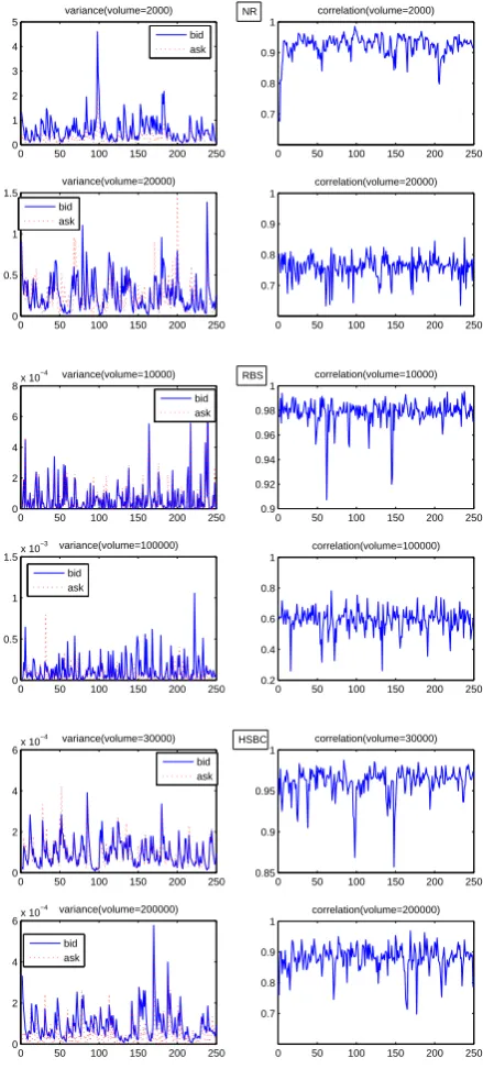
Figure 6 and 7 show the dynamic conditional correlation and the conditional variance for bid and ask position of three assets. For each asset, there are results for two different volumes. In 5 minute case, the most fluctuant correlation is the sample volume equal to 2000 of North-ern Rock, which ranges from−0.7to 1.
Table 2: Estimated Parameters at 5 minutes frequency
NR
v=2000 5 minute 10 minute
Ask Bid Ask Bid
a0 2.8047e−7 (3.6838e−8)
2.6218e−7
(3.5863e−8)
1.8026e−6
(7.8993e−5)
2.2207e−6
(5.7645e−5) a1 0.2367
(0.0121) (00..20130100) (00..18170218) (00..11360143) β1 0.7202
(0.0193) (00..75700169) (00..52550088) (00..54990087) v=10000 Ask Bid Ask Bid a0 3.6017e−7
(4.5469e−8)
4.7074e−7
(7.5653e−8)
2.1940e−6
(7.3669e−5)
2.3968e−6
(5.8352e−5) a1 0.2609
(0.0105) (00..15850131) (00..09610230) (00..18670526) β1 0.6924
(0.0187) (00.73557.0298) (00..56010940) (00..52000701) v=20000 Ask Bid Ask Bid a0 2.6298e−7
(2.6819e−8) (54..37330698ee−−8)7 (52.2782.5326ee−−5)6 (43.9412.1364ee−−5)6 a1 0.2631
(0.0087) (00..15640103) (00..16410103) (00..18360204) β1 0.7148
(0.0128) (00..76300189) (00..48380082) (00..47960068) RBS
v=10000 Ask Bid Ask Bid a0 7.6274e−7
(3.6187e−8) 1(4.2803.715ee−−8)6 (44.739.818ee−−6)6 (44.4760.3153ee−−6)6 a1 0.2706
(0.0102) (00..45800264) (00..35430016) (00..55560163) β1 0.5710
(0.0168) (00..30410204) (00..40010214) (00..00120211) v=50000 Ask Bid Ask Bid a0 1.9233e−7
(1.4278e−8) (41..46876034ee−−8)6 (15.1494.8548ee−−7)6 (14.4429.6625ee−−7)6 a1 0.3472
(0.0164) (00..61260226) (00..59280125) 0(0.77175.0258) β1 0.5736
(0.0164) (00..30410204) (00..02310168) (00..0243)064 v=100000 Ask Bid Ask Bid a0 1.376e−6
(1.9968e−5)
1.5055e−6
(4.094e−8)
4.8786e−6
(4.898e−6)
5.9844e−6
(5.094e−6) a1 0.4953
(0.0142) (00..23000201) (00..56220142) (00..57630136) β1 0.5046
(0.0106) (00..23180132) (00..30170213) (00..0332)012 HSBC
v=50000 Ask Bid Ask Bid a0 1.3154e−7
(7.0776e−9)
1.5111e−7
(7.2394e−9)
2.3042e−7
(5.0498e−7)
2.3374e−7
(5.2187e−7) a1 0.3012
(0.0168) (00..25790157) (00..40320213) (00..42550221) β1 0.6371
(0.0124) (00..64290171) (00..53440246) (00..55260165) v=100000 Ask Bid Ask Bid a0 1.0400e−7
(7.0012e−9)
1.6348e−7
(7.7124e−9)
5.1758e−7
(3.0834e−8)
3.7381e−7
(2.0726e−8) a1 0.2383
(0.0146) (00..29530152) (00..58390323) (00..42290234) β1 0.7131
(0.0182) (00..62010121) (00..40900190) (00..56300273) v=200000 Ask Bid Ask Bid a0 1.3685e−7
(7.5151e−9)
1.4553e−7
(5.9531e−9)
2.3844e−7
(5.8665e−7)
2.4243e−7
(5.9865e−7) a1 0.2781
(0.0164) (00..29320126) (00..48710244) (00..43320216) β1 0.6429
(0.0161) (00..63810126) (00..50020192) (00..55820298)
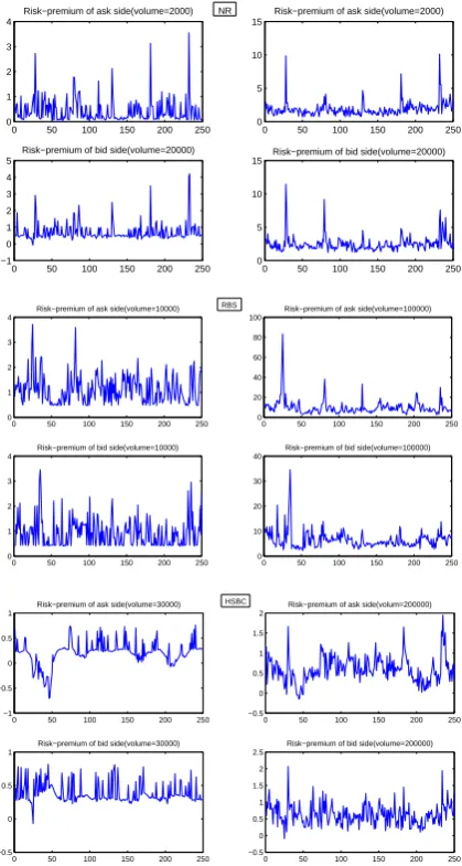
big jumps of risk premium which can effect the traders who plan to execute large volumes in short time. The risk premium also shows different with same volume but different trading positions.
Table 3 reports the liquidity risk premium of price LAIVaR for the three stocks with two different frequen-cies (5 minutes and 10 minutes). The values in brackets are the mean liquidity risk premium in percentage. The BDSS model based on the bid-ask spread only consid-ers price impact. For improvement, we propose LAIVaR model to adjust conventional VaR by incorporating si-multaneously the exogenous liquidity risk and the en-dogenous liquidity risk. The results show how the con-ventional VaR methods heavily underestimate the risk. Especially for the large volume size case, liquidity risk premium indicate a significant impact in the entire risk profile. In contract to Giot and Gramming (2006) who investigate the bid side liquidity risk premium, we are in-terested in the asymmetric effect of liquidity risk in both
Table 3: LAIVaR Risk Premia (λ).
NR
5 minutes: v=2000 v=10000 v=20000 Ask 0.3370 1.0938 1.6755 (%) (0.0005) (0.0010) (0.0014) Bid 0.8781 1.3210 2.9364 (%) (0.0008) (0.0012) (0.0025)
RBS
v=10000 v=50000 v=100000 Ask 1.9241 3.9213 9.4878 (%) (0.0011) (0.0029) (0.0048) Bid 1.3305 6.7812 11.9636 (%) (0.0007) (0.0032) (0.0054)
HSBC
v=50000 v=100000 v=200000 Ask 0.9624 1.0362 1.4567 (%) (0.0010) (0.0013) (0.0017) Bid 0.7133 0.07982 1.4827 (%) (0.0008) (0.0009) (0.0017)
NR
10 minutes: v=2000 v=10000 v=20000 Ask 0.4063 1.2894 1.8695 (%) (0.0004) (0.0011) (0.0016) Bid 0.6982 1.1995 2.4876 (%) (0.0007) (0.0010) (0.0021)
RBS
v=10000 v=50000 v=100000 Ask 1.1095 1.6382 7.012 (%) (0.0008) (0.0009) (0.0048) Bid 0.8963 3.7678 9.5969 (%) (0.0006) (0.0019) (0.0048)
HSBC
v=50000 v=100000 v=200000 Ask 0.2229 0.4780 0.6150 (%) (0.0003) (0.0005) (0.0007) Bid 0.3769 0.5975 0.6471 (%) (0.0004) (0.0007) (0.0007)
ask and bid side. Because the asymmetric information of two sides and ask side risk is also important especially for investors who are in short position. For example, the liq-uidity risk premia of different volumes for the NR stock are larger on bid side in both 5 minutes and 10 minutes cases. However in the case of RBS, the liquidity risk pre-mium of ask side is larger than bid side when the volume is high (v = 10000). For HSBC, the liquidity risk pre-mium is roughly the same on both sides. The results also show that the trend of liquidity risk premium is similar in both 5 minutes and 10 minutes frequency.
General speaking, by examining the liquidity risk pre-mium, one can reveal the liquidity risk component when measuring the VaR model. An investor, especially for the one who have to execute large size volume of asset, must take into account the effect of liquidity in order to trade more rationally.
5
Conclusion
This paper extends the conventional VaR measurement methodology by incorporating the liquidity risk of trading asset and trade positions of market participators. We use the information of limited order book data to study the asymmetric risk effect for bid and ask side.
liquid-ity risk effect to instead of the ask-bid spread. Compared with Giot and Gramming (2006), we use different real re-turn process which can reflect the real market information to measure liquidity adjusted intraday VaR (LAIVAR). Furthermore, we also proposed the asymmetric behaviors of both upside and downside LAIVaR and a liquidity risk premium in our analysis.
Our results show that the liquidity risk is a crucial factor in estimating VaR. Negligence of liquidity cost will lead to underestimation of risk as the conventional VaR model. We further contribute by studying and contrasting the patterns of LAIVaR and liquidity risk premium between bid side and ask side of an order drive stock market. We provide significant and specific information for investors who want to go long or short. Therefore, the modeling of the LAIVaR allows investors to adjust positions with a benchmark for the optimal order scheduling.
References
[1] T. Agnelidis and A. Benos. Liquidity adjusted value at risk based on the components of bid-ask spread.
Applied Financial Economics, 16(11):835–851, 2006.
[2] T. G. Andersen and T. Bollerslev. Intraday period-icity and volatility persistence in financial markets.
Journal of Empirical Finance, 4(2), 1999.
[3] A. Bangia, F. Diebold, T. Schuermann, and J. Stroughair. Modeling liquidity risk with impli-cations for traditional market risk measurement and management. The Wharton Financial Institutions Center, 1999.
[4] A. Beltratti and c. Morana. Computing value at
risk with high frequency data. Journal of Empirical
Finance, 6(5):431–455, 1999.
[5] D. Bertsimas and A. W. Lo. Optimal control of
ex-ecution costs.Journal of Financial Markets, 1(1):1–
50, 1998.
[6] F Black. Towards a fully automated exchange : Part 1. Financial Analyst Journal, 27(1):29–34, 1971.
[7] T. Bollerslev, R. Engle, and J. Wooldridge. A capital asset pricing model with time varying covariances.
Journal of Political Economy, 96(1):116–131, 1998.
[8] CGFS. Asymmetric dynamics in the correlations of global equity and bond returns. Market liquidity: research findings and selected policy implications, Basel, 2000.
[9] G. Colletaz, C. Hurlin, and S. Tokpavi. Irregularly spaced intraday value at risk (isivar) models - fore-casting and predictive abilities. Working paper, Uni-versity of Orléans, 2007.
[10] G. Dionne, P. Duchesne, and M. Pacurar. Intraday value at risk (ivar) using tick-by-tick data with ap-plication to the toronto stock exchange. Working paper, HEC Montreal, 2006.
[11] K. Dowd.Beyond Value at Risk : the New Science of
Risk Management. John Wiley and Sons., Chichester and New York, 1998.
[12] R. Engle and K. Kroner. Multivariate
simultane-ous generalized arch. Journal of Political Economy,
11(6):122–150, 1995.
[13] R. F. Engle. Dynamic conditional correlation: A simple class of generalized autoregressive conditional
heteroskedasticity models. Journal of Business and
Economic Statistics, 20(3):339–350, 2002.
[14] L. S. Erwan. Incorporating liquidity risk in var mod-els. Working Paper, University of Rene, 2001.
[15] P. Giot. Time transformations, intraday data, and
volatility models. Journal of Computational
Fi-nance, 4(2):31–62, 2000.
[16] P. Giot. Market risk models for intraday data.
The European of Journal of Finance, 11(4):309–324, 2005.
[17] P. Giot and J. Gramming. How large is liquidity
risk in an automated auction market? Empirical
Economics, 30(9):867–887, 2006.
[18] L. R. Glosten, R. Jagannathan, and D. E. Runkle.
Mopping up liquidity. Risk, 10(12):170–173, 1997.
[19] Y. Hisata and Y. Yamai. Research toward the prac-tical application of liquidity risk evaluation methods. Discussion Paper, Institute for Monetary and Eco-nomic Studies, Bank of Japan, 2000.
[20] C. Lawrence and G. Robinson. Liquidity, dynamic
hedging and value at risk. Risk Management for
Financial Institutions, 1(9):63–72, 1997.
[21] A. Madhavan, M. Richardson, and M. Roomans. Why do security prices change? a transaction-level
analysis of nyse stocks. Review of Financial Studies,
10(4):1035–1064, 1997.
[22] J.P. Morgan. Morgan technical document. Fourth Edition, 1996.
[23] Shouyang W Yiongmiao H Yi L Xiangli L, Siwei C. An empirical study on information spillover effects between the chinese copper futures market and spot
market.Physica A: Statistical Mechanics and its
0 10 20 30 40 50 60 70 80 90 100 1130
1135 1140 1145 1150 1155 1160 1165
NR
v=2000(upside) v=20000(upside) Mid−price(upside) v=2000(downside) v=20000(downside) Mid−price(downside) v=10000(upside) v=10000(downside)
0 10 20 30 40 50 60 70 80 90 100 1920
1930 1940 1950 1960 1970 1980 1990 2000 2010 2020 2030
RBS
v=10000(upside) v=100000(upside) Mid−price(upside) v=10000(downside) v=100000(downside) Mid−price(downside) v=50000(upside) v=50000(downside)
0 10 20 30 40 50 60 70 80 90 100 880
882 884 886 888 890 892 894 896 898 900
HSBC
[image:9.595.70.283.131.627.2]v=50000(upside) 200000(upside) Mid−price(upside) v=50000(downside) v=200000(downside) Mid−price(downside) v=100000(upside) v=100000(downside)
Figure 4: Price IVaR (α=5%) of three companies with 5 minutes sampling frequency
0 10 20 30 40 50 60 70 80 90 100 1145
1150 1155 1160 1165 1170 1175 1180 1185 1190 1195 1200
NR
v=2000(upside) v=20000(upside) Mid−price(upside) v=2000(downside) v=20000(downside) Mid−price(downside) v=10000(upside) v=10000(downside)
0 10 20 30 40 50 60 70 80 90 100 1960
1980 2000 2020 2040 2060 2080
RBS
v=10000(upside) v=100000(upside) Mid−price(upside) v=10000(downside) v=100000(downside) Mid−price(downside) v=50000(downside) v=50000(upside)
0 10 20 30 40 50 60 70 80 90 100 880
885 890 895 900 905 910 915 920
HSBC
v=30000(upside) v=200000(upside) Mid−price(upsde) v=30000(downside) v=200000(downside) Mid−price(downsde) v=100000(downside) v=100000(upside)
[image:9.595.325.539.151.624.2]0 100 200 300 400 0 1 2 3 4 5 variance(volume=2000)
0 100 200 300 400 −1 −0.5 0 0.5 1 correlation(volume=2000)
0 100 200 300 400 0 1 2 3 4 variance(volume=20000)
0 100 200 300 400 0.4 0.5 0.6 0.7 0.8 0.9 correlation(volume=20000) bid ask bid ask NR
100 200 300 400 0
0.2 0.4 0.6 0.8
1x 10
−4 variance (volume=10000)
0 100 200 300 400 0.8 0.85 0.9 0.95 1 correlation(volume=10000)
0 100 200 300 400 0
2 4 6x 10
−4 variance(volume=100000)
0 100 200 300 400 0 0.2 0.4 0.6 0.8 correlation(volume=100000) bid ask RBS
0 100 200 300 400 0
0.5 1 1.5 2x 10
−5 variance(volume=200000)
0 100 200 300 400 0.65 0.7 0.75 0.8 0.85 0.9 0.95 1 correlation(volume=200000) bid ask
0 100 200 300 400 0
0.5 1 1.5 2 2.5x 10
−5 variance(volume=50000)
[image:10.595.49.281.133.638.2]0 100 200 300 400 0.65 0.7 0.75 0.8 0.85 0.9 0.95 1 correlation(volume=50000) HSBC
Figure 6: Variance and correlation with different volume sizes for 5 minutes sampling frequency
0 50 100 150 200 250 0 1 2 3 4 5 variance(volume=2000)
0 50 100 150 200 250 0.7
0.8 0.9 1
correlation(volume=2000)
0 50 100 150 200 250 0
0.5 1 1.5
variance(volume=20000)
0 50 100 150 200 250 0.7 0.8 0.9 1 correlation(volume=20000) bid ask bid ask NR
0 50 100 150 200 250 0
2 4 6 8x 10
−4 variance(volume=10000)
0 50 100 150 200 250 0.9 0.92 0.94 0.96 0.98 1 correlation(volume=10000)
0 50 100 150 200 250 0
0.5 1 1.5x 10
−3 variance(volume=100000)
0 50 100 150 200 250 0.2 0.4 0.6 0.8 1 correlation(volume=100000) bid ask bid ask RBS
0 50 100 150 200 250 0
2 4 6x 10
−4 variance(volume=30000)
0 50 100 150 200 250 0.85
0.9 0.95 1
correlation(volume=30000)
0 50 100 150 200 250 0
2 4 6x 10
−4 variance(volume=200000)
0 50 100 150 200 250 0.7 0.8 0.9 1 correlation(volume=200000) bid ask bid ask HSBC
[image:10.595.330.550.146.633.2]0 100 200 300 400 0
1 2 3 4
Risk−premium of ask side(volume=2000)
0 100 200 300 400 0
2 4 6 8 10 12
Risk−premium of ask side(volume=20000)
0 100 200 300 400 0
1 2 3 4 5
Risk−premium of bid side(volume=2000)
0 100 200 300 400 0
2 4 6 8 10
Risk−premium of bid side(volume=20000) NR
0 100 200 300 400 −20
−10 0 10 20
Risk−premium of bid side(volume=10000)
0 100 200 300 400 −20
0 20 40 60
Risk−premium of bid side(volume=100000) 0 100 200 300 400
0 1 2 3 4 5
Risk−premium of ask side(volume=10000)
0 100 200 300 400 0
10 20 30 40 50 60
Risk−premium of aks side(volume=100000) RBS
0 100 200 300 400 0
1 2 3 4
Risk−premium of ask side(volume=50000)
0 100 200 300 400 0
1 2 3 4 5 6
Risk−premium of ask side(volume=200000)
0 100 200 300 400 0
0.5 1
1.5 Risk premium of bid side(volume=50000)
0 100 200 300 400 0
1 2 3 4 5
[image:11.595.73.275.187.583.2]6 Risk−premium of bid side(volume=200000) HSBC
Figure 8: Risk-premium with 5 minutes sampling fre-quency and different volume sizes
0 50 100 150 200 250 0
1 2 3 4
Risk−premium of ask side(volume=2000)
0 50 100 150 200 250 0
5 10 15
Risk−premium of ask side(volume=2000)
0 50 100 150 200 250 −1
0 1 2 3 4 5
Risk−premium of bid side(volume=20000)
0 50 100 150 200 250 0
5 10 15
Risk−premium of bid side(volume=20000) NR
0 50 100 150 200 250 0
1 2 3 4
Risk−premium of ask side(volume=10000)
0 50 100 150 200 250 0
20 40 60 80 100
Risk−premium of ask side(volume=100000)
0 50 100 150 200 250 0
1 2 3 4
Risk−premium of bid side(volume=10000)
0 50 100 150 200 250 0
10 20 30 40
Risk−premium of bid side(volume=100000) RBS
0 50 100 150 200 250 −1
−0.5 0 0.5 1
Risk−premium of ask side(volume=30000)
0 50 100 150 200 250 −0.5
0 0.5 1 1.5 2
Risk−premium of ask side(volum=200000)
0 50 100 150 200 250 −0.5
0 0.5 1
Risk−premium of bid side(volume=30000)
0 50 100 150 200 250 −0.5
0 0.5 1 1.5 2 2.5
Risk−premium of bid side(volume=200000) HSBC
[image:11.595.332.542.191.584.2]