Movement Detection and Moving Object
Distinction Based on Optical Flow
Paulo A. S. Mendes
†, Mateus Mendes
†∗, A. Paulo Coimbra
†, Manuel M. Cris´ostomo
†Abstract—Detection of moving objects in sequences of images is an important research field, with applications for surveillance, tracking and object recognition among others. An algorithm to estimate motion in video image sequences, with moving object distinction and differentiation, is proposed. The motion estimation is based in three consecutive RGB image frames, which are converted to gray scale and filtered, before being used to calculate optical flow, applying Gunnar Farneb¨ack’s method. The areas of higher optical flow are maintained and the areas of lower optical flow are discarded using Otsu’s adaptive threshold method. To distinguish between different moving objects, a border following method was applied to calculate each object’s contour. The method was successful detecting and distinguishing moving objects in different types of image datasets, including datasets obtained from moving cameras.
Index Terms—Computer Vision, Movement Detection, Opti-cal Flow, Object Detection.
I. INTRODUCTION
N
OWADAYS, more than ever, it is possible the develop-ment and application of more complex algorithms using inexpensive hardware. Optical flow and image processing in general are computationally demanding. Nonetheless, they are already possible in real time using common hardware.Optical flow is an important method for motion estima-tion in visual scenes. Lucas and Kanade image registraestima-tion method, also known as gradient-based optical flow, makes motion estimation in images possible with very fast com-putation [1], [2]. Pyramidal Lucas and Kanade [3], Gunnar Farneb¨ack [4], [5], [6] and Brox et al. [7] optical flow are other methods for motion estimation in images.
Sengar and Mukhopadhyay developed excellent methods to detect movement [8] and a moving object area [9], based on optical flow. The methods show precise results with low processing time, which is important for automatic surveil-lance and the detection of moving objects using computer vision. The method creates a smaller image, which is a fraction of the original image, and contains a representation of the moving objects detected. When there are multiple moving objects the image returned contains all the objects and requires further processing to distinguish between the objects.
Chen and Lu proposed object-level motion detection from a moving camera [10], estimating the objects’ movement relative to the camera.
The present paper describes a method of motion estimation based on Gunnar Farneb¨ack’s optical flow. The aim is to calculate a dense optical flow from consecutive images to
∗Polytechnic Institute of Coimbra - ESTGOH, Portugal. E-mail:
†ISR - Institute of Systems and Robotics, Dept. of Electrical
and Computer Engineering, University of Coimbra, Portugal. E-mail: [email protected], [email protected], [email protected].
accomplish the most precise movement detection in the least amount of time. Images are preprocessed, namely converted to gray scale and smoothed to improve the results. Otsu’s threshold method [11] is applied to create a binary image representing the areas of larger optical flow. Suzuki and Abe’s border following method [12] is applied to the binary image to make the distinction of different moving objects.
The paper presents results of different experiments using images selected from popular datasets, each one representing particular challenges for optical flow calculation.
Section II describes the hardware, the software and the datasets used. The main steps of the algorithm are described in Section III. The tests and results are presented and discussed in Section IV and Section V. Section VI draws some conclusions and possible future developments.
II. EXPERIMENTAL SETUP
1) Hardware: The hardware used was a laptop with a 2.40 GHz Intel Core i7-3610QM processor, 6 GB RAM and a NVIDIA Graphics Processing Unit (GPU) with 2 GB memory and 96 CUDA cores.
2) Datasets: The proposed methodology were tested us-ing images from datasets adequate for optical flow calcu-lation. The first experiments were performed using images from dataset “O SM 02” from LASIESTA Database, of the Universidad Polit´ecnica de Madrid [13], which contains outdoor images of moving people taken with a moving camera. The camera resolution is 352×288 pixels. Other datasets used are LASIESTA Database “O SM 07” and Freiburg University “Chinese Monkey” [14].
3) Software: The algorithms were coded in C and C++ language using OpenCV (Open Source Computer Vision Library) [15]. OpenCV, originally developed by Intel, is a software toolkit for processing real-time image and video, that also provides analytics and machine learning capability. It is free for academic and commercial use.
For a better result, part of the algorithm, was developed using OpenCV CUDA module. OpenCV CUDA module is a set of classes and functions to utilize CUDA computational capabilities.
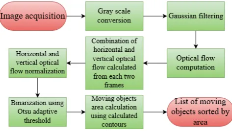
Fig. 1. System architecture with input images from a camera or an HDD and the system output (list of moving objects sorted by area).
Fig. 2. Steps of the algorithm to detect moving objects.
future applications of moving object detection possible in real time. The algorithm to detect moving objects is represented in the flow chart shown in Figure 2. This will be explained in Section III.
III. MOVING OBJECTS DETECTION
Motion estimation is based on three consecutive RGB frames (F1, F2 and F3), as shown in Figure 3. These
images will be preprocessed and then used for optical flow calculation as presented next.
A. Conversion to gray scale
The three RGB frames are first converted to gray scale images. The conversion is made using Equation 1, giving different weights to each color channel. The weights are the default OpenCV values.
Grayi(x, y) = 0.299Ri(x, y)+0.587Gi(x, y)+0.114Bi(x, y)
(1)
Ri, Gi and Bi are the red, green and blue channel
com-ponents of RGB frame Fi. The pixel position in the frame
(a) FrameF1 (b) FrameF2 (c) FrameF3
Fig. 3. Three consecutive RGB frames from LASIESTA Database.
[image:2.595.304.547.169.249.2](a) FrameGray1 (b) FrameGray2 (c) FrameGray3
Fig. 4. Gray scale images obtained from the RGB frames shown in Figure 3.
(a) FrameSmooth1 (b) FrameSmooth2 (c) FrameSmooth3
Fig. 5. Gray scale frames filtered with Gaussian filter.
image is defined by coordinates (x, y). Figure 4 shows the same images as Figure 3 after gray scale conversion, using Equation 1.
B. Noise smoothing
Digital images usually have some noise. To minimize that problem, a Gaussian filter is applied to each frame using the two dimensional Gaussian function shown in Equation 2.
Gaussian(x, y) = 1 2πσ2e
−(x2 +y2 )
2σ2
(2)
The resulting Gaussian distribution resembles a bell curve which is used to smooth the image. The standard deviation of the Gaussian filter distribution,σ, can be interpreted as a measure of its size, controlling the bell curve aperture. The Gaussian distribution is approximated to a suitable convolu-tion kernel (a matrix composed of floating point values). To obtain the smoothed image it is necessary to convolve the Gaussian filter with the gray image. The convolution follows Equation 3, using the convolution kernel that results from a chosenσ value.
Smoothi(x, y) =Gaussian(x, y)∗Grayi(x, y) (3)
The kernel size was chosen to be of3×3for fast computation applying the filter.
The optimal value for the standard deviation, σ, varies from image to image. However, its calculation takes time. In the present work was used a constant valueσ= 1.5 that showed good results in the experiments. Figure 5 shows the results obtained after filtering the images shown in Figure 4, using Equation 3.
C. Optical flow computation
Optical flow output is a two dimensional (2D) field that represents moving objects in the real world or a moving camera taking frames of a scene. In computer vision, the main method for motion estimation is optical flow. It is also used in the present paper.
[image:2.595.50.287.236.370.2] [image:2.595.45.293.686.766.2](a) Farneb¨ack method (b) Broxet al.method (c) Pyramidal Lucas and Kanade method
Fig. 6. Resulting movement detection using different optical flow methods.
[image:3.595.303.551.52.165.2](a)h1 (b)v1
Fig. 7. Optical flow in horizontal and vertical directions (h1 andv1),
calculated between framesF1andF2.
Brox et al. optical flow outperforms the other methods in precision. However, it also requires more processing time. Since the aim of the present work is to apply the developed algorithm in real time, Broxet al.optical flow was discarded. Farneb¨ack’s method was also tested. It is faster than Pyra-midal Lucas and Kanade. It showed the best results, in a precision to computation time ratio basis. Figure 6, shows the images of the optical flow obtained for these methods applied to the sequence of images of Fig. 5. Table I shows the computation times measured to calculate the optical flow among three consecutive images—that is to calculate the optical flow between framesF1-F2 and between framesF2 -F3. The aim of the present work is to detect movement
in a sequence of images. Therefore, a dense optical flow calculation is applied for every two consecutive frames, using Gunnar Farneb¨ack’s method.
The optical flow calculation results in horizontal and vertical directions optical flow images as shown in figures 7 and 8. Figure 7 and Figure 8 show vertical and horizontal optical flows calculated using, respectively, the first and second frames and second and third frames shown in Figure 5. The optical flow pixels are a projection of the motion field onto the 2D image. The motion field is a representation of the real3D world motion.
[image:3.595.47.293.53.133.2](a)h2 (b)v2
Fig. 8. Optical flow in horizontal and vertical directions (h2 andv2),
calculated between framesF2andF3.
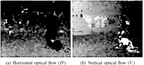
[image:3.595.46.292.171.283.2](a) Horizontal optical flow (H) (b) Vertical optical flow (V)
Fig. 9. Sum of horizontal and vertical optical flows applying equations 4 and 5 to the images shown in Figures 7 and 8.
D. Optical flow directions combination
For each two filtered consecutive frames there are the horizontal and vertical optical flow components, hi andvi, as explained above. Therefore, three consecutive frames (F1, F2 and F3) result in four optical flow images (h1, v1, h2
and v2). The horizontal and vertical components are then
added resulting into one single image for each optical flow direction, as shown in equations 4 and 5.
H(x, y) =h1(x, y) +h2(x, y) (4)
V(x, y) =v1(x, y) +v2(x, y) (5)
H andV are the images of horizontal and vertical optical flow and(x, y)are the pixel coordinates. Figure 9 shows the results of applying equations 4 and 5 to the images shown in Figures 7 and 8. The magnitude of the horizontal and vertical optical flows is calculated applying Equation 6.
M(x, y) =pH2(x, y) +V2(x, y) (6)
The resulting optical flow, obtained after applying Equation 6 to imagesH andV, consists of one single 2D gray scale image (M), as shown in Figure 10(a).
The pixel’s values in M do not occupy all the range of the gray scale images ([0,255]for 8-bit gray scale images). Therefore, for a better result, the image M is normalized using Equation 7.
N(x, y) = M(x, y)−M min
Mmax−Mmin ×Imax (7)
In the equation,M(x, y)is the optical flow magnitude value at pixel position(x, y).Mmin andMmax are the minimum
and maximum values in the image M. Finally, N(x, y), is the normalized optical flow at pixel position (x, y) and
Imax is the maximum possible pixel value (255 for 8
-bitgray scale images). Normalization facilitates the motion estimation procedure because of the wider range to calculate the optimal threshold value, as explained in next Section.
E. Movement detection using adaptive threshold
The normalized optical flow image (N) contains noise (detected “false movement”). Noise which was not com-pletely eliminated by the preprocessing of the original RGB frames (F1, F2 andF3) causes “false movement” detection
[image:3.595.48.293.645.757.2]“Chinese Monkey” set 0.144000 1.887000 0.491800 720×432
[image:4.595.47.490.83.269.2](a) Optical flow magnitude (M) (b) Normalized optical flow magni-tude (N)
Fig. 10. Optical flow magnitude following Equation 6 and normalized optical flow following Equation 7.
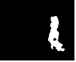
Fig. 11. Binarized image obtained applying Otsu’s threshold method to the image of the Figure 10(b). The white area corresponds to the detected movement.
method consists in computing the gray scale image his-togram, and determining the optimal threshold value based on the histogram peaks. The threshold is chosen as a value between two peaks of a bimodal image histogram. The pixel values above the threshold value are set to one and the values below the threshold are set to zero.
Xu, Jin and Song refer that the threshold method is effective to separate objects from the background when the gray levels are substantially different between them [16]. Optical flow normalization, as described in Section III-D, facilitates this task.
In the present work the threshold value, defined as λ, is calculated from the normalized optical flow image (N). Afterwards, the image is binarized applying Equation 8.
B(x, y) =
1 if N(x, y)≥λ
0 otherwise (8)
The binarized image (B) resulting from applying Equation 8 to imageN is shown in Figure 11. The white areas identify the areas of movement detected in the original sequence of three images. The black areas are areas where there is no movement detected.
F. Moving object area detection
For a better distinction of the moving objects, the objects’ contours are calculated from the binary image (B) and stored
Fig. 12. Calculated contours from the binary image. The largest contour corresponds to a6342.5pixelsand the smaller to only0.5pixelsarea.
in a data structure (as a contour list). Figure 12 shows the two contours calculated from image B and drawn in a black background image. The contours are determined using Suzuki and Abe’s border following method [12].
The list of contours contains small contours which are most likely noise. Therefore, the small contours are ignored. The area of all contours is calculated and only the contours which have an area larger than a predefined value are considered. Those contours represent some object (or part of one) moving in the real world. On the other hand, the contours with area smaller than the predefined value are too small to be relevant. In the present implementation, only the largest area contour is selected.
The area of the largest contour shown in Figure 12 is
6342.5 pixels. It was calculated using Green’s theorem1
OpenCV implementation.
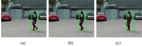
Knowing the moving objects’ contours, the corners of the minimum rectangle that contains those contours are calculated and the rectangle is marked in the original image, detecting the region of interest (ROI). Figure 13, shows a green rectangle over the ROI in the original RGB frames. The ROI cut out from each RGB frame can be seen in Figure 14.
Figure 15 shows the moving person superimposed, cut out by hand, on the area of movement detected for comparative reasons. As the images show, the area where movement was detected contains approximately the union of the areas the person occupied in the three images. There is an extra area to the bottom right of the image which corresponds to part of the person’s shadow, which also moved.
IV. RESULTS WITH OTHER SETS OF IMAGES
[image:4.595.109.232.308.409.2](a) (b) (c)
Fig. 13. Region of interest marked in green in the original RGB frames (F1,F2andF3) used to detect movement.
(a) (b) (c)
Fig. 14. Cut out region of interest from the largest area contour calculated, from each LASIESTA Database RGB frame.
A. Images from LASIESTA Database
Figure 16 shows another set of frames from LASIESTA Database, which is an outdoor set with different types of camera motion. This set has medium camera jitter and low camera rotation. Figure 16(d) shows the binarized image presenting the detected movement areas. It is clear from this result that this set is difficult. Since the camera is non-static, not only the persons are moving but also the static objects in the scene. The threshold method eliminates the slow moving objects, but even so there are many areas with detected move-ment in the binary image. In these three frames sequence 97 contours were identified. These contours are shown in Figure
1Green’s theorem brief explanation: https://en.wikipedia.org/wiki/Green’s
theorem (last checked 16.08.2018).
(a) Human figure superimposed on FrameF1
(b) Human figure superimposed on FrameF2
(c) Human figure superimposed on FrameF3
[image:5.595.122.217.169.258.2](d) Overlap of the three frames
Fig. 15. Image of the human figure moving-object superimposed on the area of movement detected, for each frame.
16(e). The areas of the three largest contours calculated using Green’s theorem are 24325.5 (yellow), 5006.0 (cyan) and
2060.0(pink)pixels. These contours results in the ROI seen in Figures 16(f), 16(g) and 16(h) respectively.
B. Images from Freiburg Chinese Monkey dataset
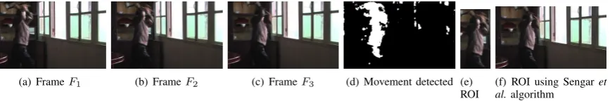
Figure 17 shows three consecutive RGB frames from Freiburg university, the Chinese Monkey dataset. The Chi-nese Monkey dataset is a hard one because of the fast camera movement. The camera movement causes areas of motion in the image where there are only static objects.
Since the algorithm applied to calculate the ROI was the contour of the largest area, the resulting ROI is only the area where there is a person, as shown in Figure 17(e). In this case the algorithm developed to differentiate regions of movement is more effective selecting the region of interest than the algorithm developed by Sengar and Mukhopadhyay as mentioned in Section I. Using Sengar et al.’s method of movement detection, the result is almost all the original image frame, since there are regions of strong optical flow all over the analysed images, as shown in Figure 17(f).
C. Computation time
The methodology described in Section III was tested with the CPU and GPU capabilities, applied to the LASIESTA “O SM 02” dataset. The total execution time measured, using the CPU, is of 114.218 milliseconds (in the best of three different runs). The total execution time measured, using the GPU, is of 61.591 milliseconds (in the best of three different runs).
V. DISCUSSION
Some surfaces, like metal grilles, are difficult for optical flow calculation. They result in false movement detection. In the present work the problem was minimized by applying a Gaussian filter as described in Section III-B.
As shown in Section III-C, Gunnar Farneb¨ack’s optical flow calculation method shows good results within accept-able calculation time. That makes it appropriate for surveil-lance purposes where near real time processing is necessary. Otsu’s method is a good choice for the calculation of the normalized optical flow threshold value. There are several improvements to that same method that could be applied in future work [16].
As described in Section III-E the threshold method is very important to reduce false movement detection (noise due to difficult surfaces on real world or a larger movement of the camera). The more correct the threshold value the more precise the movement detection will be.
[image:5.595.46.293.505.605.2] [image:5.595.45.292.633.741.2](a) FrameF1 (b) FrameF2 (c) FrameF3 (d) Movement detected (e) Contours of detected
movement areas
(f) ROI 1 (g) ROI 2
(h) ROI 3
Fig. 16. LASIESTA Database RGB image set (“O SM 07”): (a-c) consecutive RGB frames used, (d) binarized image of movement detection, (e) contours of moving object areas and (f-h) regions of interest of movement detect (from the three largest area contours).
(a) FrameF1 (b) FrameF2 (c) FrameF3 (d) Movement detected (e)
ROI
[image:6.595.52.550.52.140.2](f) ROI using Sengaret al.algorithm
Fig. 17. Freiburg Database RGB image set (“Chinese monkey”): (a-c) consecutive RGB frames used, (d) binarized image of movement detected and (e) region of interest from movement detection obtained with proposed methodology and (f) obtained using Sengaret al.algorithm.
VI. CONCLUSION
A new methodology capable of detecting different mov-ing objects usmov-ing Gunnar Farneb¨ack’s optical flow, Otu’s adaptive threshold and Suzuki and Abe’s contour calculation method is presented. The methodology was successful in detecting distinct moving objects in images from static and moving cameras. Regions of the image can then be selected based on the moving objects’ contour areas.
Experiments using images from different datasets show that the methodology is effective and fast enough to be used in real time. Therefore, it is suitable to use in applications such as surveillance, object tracking, object counting and others applications.
Future work includes development of an optimal Gaussian filter calculator for gray scale images, in order to get a better optical flow precision.
Otsu’s threshold method can also be improved, as dis-cussed in Section V. The process can also be sped-up using parallel GPU computation. As mentioned in Section V, it is possible to use another optical flow calculation method to achieve even better precision on the movement detection at the cost of additional calculation time.
ACKNOWLEDGMENT
This work has been supported by OE - national funds of FCT/MCTES (PIDDAC) under project UID/EEA/00048/2019.
REFERENCES
[1] B. D. Lucas and T. Kanade, “An iterative image registration technique with an application to stereo vision,”International Joint Conference on Artificial Intelligence (7th), vol. 2, pp. 674–679, 1981.
[2] A. Faria, “Fluxo ptico,”ICEx-DCC-Viso Computacional, 1992. [3] J.-Y. Bouguet, “Pyramidal implementation of the affine Lucas Kanade
feature tracker description of the algorithm,”Intel Corporation, vol. 10, 2000.
[4] G. Farneb¨ack, “Two-frame motion estimation based on polynomial expansion,”Scandinavian Conference on Image Analysis, pp. 363– 370, 2003.
[5] G. Farneb¨ack, “Polynomial expansion for orientation and motion estimation,” PhD dissertation, Department of Electrical Engineering, Link¨oping University, Sweden, 2002.
[6] Gunnar Farneb¨ack, “Fast and accurate motion estimation using orienta-tion tensors and parametric moorienta-tion models,”International Conference on Pattern Recognition. ICPR-2000, vol. 1, pp. 135–139, 2000. [7] T. Brox, A. Bruhn, N. Papenberg, and J. Weickert, “High accuracy
optical flow estimation based on a theory for warping,”Lecture Notes in Computer Science, vol. 3024, pp. 25–36, 2004.
[8] S. S. Sengar and S. Mukhopadhyay, “Detection of moving objects based on enhancement of optical flow,”Optik, vol. 145, pp. 130-141, vol. 145, pp. 130–141, 2017.
[9] S. S. Sengar and S. Mukhopadhyay, “Moving object area detection using normalized self adaptive optical flow,”Optik, vol. 127, no. 16, pp. 6258–6267, 2016.
[10] T. Chen and S. Lu, “Object-level motion detection from moving cameras,”IEEE, vol. 27, no. 11, pp. 2333–2343, 2017.
[11] N. Otsu, “A threshold selection method from gray-level histograms,”
IEEE Transactions on Systems, Man, and Cybernetics, vol. 9, no. 1, pp. 62–66, 1979.
[12] S. Suzuki and K. Abe, “Topological structural analysis of digitized binary images by border following,”Computer Vision, Graphics, and Image Processing, vol. 30, no. 1, pp. 32 – 46, 1985.
[13] T. Brox, A. Bruhn, N. Papenberg, and J. Weickert, “Labeled dataset for integral evaluation of moving object detection algorithms: Lasiesta,”
Computer Vision and Image Understanding, vol. 152, pp. 103–117, 2016.
[14] T. Brox and J. Malik, “Large displacement optical flow: descriptor matching in variational motion estimation,” IEEE Transactions on Pattern Analysis and Machine Intelligence, vol. 33, no. 3, pp. 500–513, 2011.
[15] OpenCV, “Open Source Computer Vision Library,” https://opencv.org/ (last checked 16.08.2018), August 2018. [16] X. Xu, S. Xu, L. Jin, and E. Song, “Characteristic analysis of Otsu
threshold and its applications,” Pattern Recognition Letters, vol. 32, no. 7, pp. 956–961, 2011.
[image:6.595.84.518.177.249.2]