Does the Stochastic Specification of the Linear
Expenditure System Matter?*
Abstract: When “income” in a system of demand equations is defined as total expenditure, actual expenditure on any commodity must lie between zero and income, or equivalently, budget shares must lie between zero and one. But models for expenditures or shares are often the sum of deterministic components (predicted values), which are functions of prices and income, and disturbances, usually assumed multivariate normal. The predicted values ought to satisfy the same bounds as the dependent variables and will do so if the demand system is “regular”. But even then, the situation is theoretically inconsistent with unbounded disturbances and it has been proposed (Fry et al., 1996) that analysis be appropriately modified. In assessing how much practical difference this makes, the linear expenditure system (LES) is, for reasons described in the paper, the crucial case. We compare estimation methods for the LES, using Irish data from 1979-99 on some broadly defined commodities, and find that the differences are not of practical concern.
I INTRODUCTION
W
hen income, y, in a system of demand equations is defined as total expenditure Σpjqj,where qi and piare the quantity and price of the ith commodity, it is obvious that the actual expenditure on any commodity must lie between zero and y, or equivalently, budget shares must lie between zero and one. However, such systems are usually modelled by the sets of n equationspiqi= fi(p, y) + ei, (1)
or
23
*We thank anonymous referees for comments leading to substantial improvements to the paper.
DENIS CONNIFFE
NIRSA and NUI, Maynooth
JOHN EAKINS
wi= gi(p, y) + ui, (2)
where wi is the i th budget share and there are n commodities.1Clearly, the
deterministic components fi and gi of these models ought to conform to the
constraints and will if the demand system is globally regular,2but even then
the usual assumptions made about the stochastic disturbances eiand ui– that
they are randomly drawn from a multivariate normal distribution – are evidently not precisely appropriate. For example, wiin (2) cannot exceed unity,
but even with a gibelow unity, a uidrawn from a normal distribution, with its infinite range, could possibly result in a sum greater than unity and hence inconsistency between the left and right hand sides of (2). Of course, in practice, the fitted multivariate normal might well have variances so small that the probability of a uibeing so large might be negligible and it is probably on this presumption that authors have usually ignored the problem.
If the deterministic components do not automatically conform to the constraints, the likelihood of difficulties is far greater. For example, an equation for a single good of the form3
y p
w= a+ bylog — + bp log — + u, (3) d1 d2
where d1 and d2 are price deflators, must, as y increases, inevitably either exceed unity or become less than zero, depending on whether by is positive or
negative. For this and other reasons, Conniffe (1993) argued that a logistic transformation of the budget share should replace win (3) giving
w y p
log —–— = a + bylog — + bplog — + v (4) 1 – w d1 d2
Now the dependent variable can take any positive or negative values like the deterministic part of the right hand side. The model is also far more compatible with a normality assumption for v, since the dependent variable can, theoretically, range from –∞ to +∞, but the motivation for (4) was
1Only n–1 of each set of equations are linearly independent because of the adding up condition of Σpjqj=y for (1), or Σwj= 1 for (2).
2Systems are globally regular if they meet the demand theory conditions implied by utility
maximisation (subject to a budget constraint) for all prices and income, although for practical purposes “all” can be relaxed to “all relevant”. Regularity implies constraints on the parameters of the utility function, but even so, few demand systems are regular for all relevant prices and incomes.
3This is the Working (1943) or Leser (1963) form, which becomes Deaton and Muellbauers’ (1980)
principally4 the incompatibility of the dependent variable and the
deterministic term in (3).
Fry, Fry and McLaren (1996) discuss the treatment of stochastic terms in the estimation of regulardemand systems, when the gi in (2) are sure to be
between zero and unity, and argue for estimation of the n-1 equation model
wi gi
log —– = log —– + vi, (5)
wn gn
instead of (2), assuming multivariate normality of the vi. (The choice of the
n th good for the denominator is arbitrary.) From a data analysis viewpoint, it is undeniable that multivariate normality is a more plausible operational assumption if choosing model (5) rather than model (2), for the reasons already stated in the case of (4). More theoretically, if we visualise (5) as the true model generating the wi, it is clear that they will lie between zero and
unity. So it is appealing to work with the form (5) and to suspect there could have been errors introduced by failure to do so in the past. That need not mean that research with the forms (1) or (2) has to have been seriously incorrect; that will depend on the importance of the stochastic specification in estimating the demand system.
In fact, many of the commonly employed demand systems, such as the AIDS model, do not satisfy (near) global regularity5and for them the form (5) could
be quite unsuitable, as Fry et al., appreciated, because the gi might not be
appropriately bounded. The linear expenditure system (LES) and the indirect addilog system are the only (near) globally regular systems (given essential constraints on the parameters) that have been frequently employed in applications. As regards the indirect addilog system, it has always been estimated in the form (5) anyway, not (at least explicitly) because of concern about the formulation of the stochastic terms, but because it was computationally convenient to do so.6 So this paper will focus on how LES
estimation is affected by the choice of (5) rather than (1) or (2).
It is true that regularity is not the only property a widely applicable
4Utility theory justification for (4) follows from considering it a two equation case (a commodity
and all other commodities, so that w2= 1 – w1) of Houthakker’s (1960) indirect addilog system. 5There have been considerable efforts to find other systems with better regularity properties
including Barnett (1983), Barnett and Lee (1985) and Chalfant (1987). Fry et al. (1996) mention the MAIDS system of Cooper and McLaren (1992), which has been applied by Boyle (1996). However, the statement remains true for the systems predominantly employed.
y y
6The indirect addilog equations have the form w
i= γi—pβi /
Σ
γj —βjand it is clear that dividing i j pjdemand system should possess and it is desirable that it be capable of modelling a wide range of conceivably observable consumer behaviour. As is pointed out in many textbooks, the regular LES lacks flexibility in this regard, partly because it is quite parsimonious in parameters. For example, the model precludes inferior goods and the occurrence of complementarity between commodities. The LES is really only appropriate for a set of very broadly defined commodities. However, even with these reservations, the LES is an important system. It has been popular with Irish researchers since the seventies (Casey, 1973; O“Riordan, 1976; McCarthy, 1977) and it is still employed. For example, the ESRI (Duffy et al.,2001) review and forecast of the Irish economy was based on methodology incorporating an LES for the household consumption sector.
II ESTIMATING THE LES
The LES is usually considered in expenditure form
piqi= γi pi+ βi(y – Σγj pj) + ei, (6)
where regularity is assured if γi are positive, βi positive and adding to unity
over the n commodities and y> Σγj pj. Sometimes the budget share form
γi pi Σγj pj
wi = —— + y yβi
1 – —–—+ ui (7)is employed. In either case, the n th equation can be omitted at the estimation stage (and deduced from the adding up condition) to avoid singularity. However, this is not the only way to proceed. Working with the n-1 equations
wi piqi γi pi + βi(y – Σγj pj)
––– = —— = ———————————— + ui*, (8)
wn pnqn γnpn+ (1 – Σnβj)(y – Σγj pj)
where Σn denotes summation excluding j = n, or the equations
wi γi pi + βi(y – Σγj pj)
log —– = log
—–———–——————— + vi (9)wn γnpn+ (1 + Σnβj)(y – Σγj pj)
The model (8) is a “half-way house” between (9) and the more familiar LES specifications, but it is worth including for completeness.
Maximum likelihood has been, and remains, the dominant estimation method in applied economics and by far the most frequent assumption about the likelihood is that it is multivariate normal. Indeed, many econometric packages do not permit any other assumption when providing estimation routines for non-linear systems of equations. Systems (6), (7), (8) and (9) are really identical as regards deterministic components, but as they differ in how the stochastic and deterministic components combine, estimation involves the maximisation of rather different likelihoods for each case. So it is reasonable to think that estimates of coefficients could be affected to some degree, in terms of bias or precision or both, by the choice of model, and it is interesting to see if this will matter in practice.
One obvious approach to comparing (6), (7), (8) and (9) would be through a simulation study, generating the data from exact LES equations for the deterministic components and combining samples from an exact multivariate normal for the stochastic components, and then comparing the distributions of estimates of the parameters. To at least some extent it is intuitively clear what would result. If the variance matrix of the multivariate normal is “small” (in the sense that the diagonal terms are) so that deterministic components greatly outweigh the stochastic components, there will be no difference, while if the reverse holds, there will be. But this is not satisfactory as a practical assessment. No one believes that consumer demand is precisely represented, even as regards deterministic components, by the LES – at best it is a reasonable approximation for some broad commodities. Nor would anyone believe that with real-world data, exact multinormality is at all plausible. What matters for practical purposes is whether choice of (6), (7), (8) or (9) makes any difference with the sort of data set typically analysed by applied economists.
III DATA AND ANALYSES
Time series of domestic expenditures on commodities at current and constant prices are available from the Irish Central Statistics Office’s National
Income and Expenditure Accounts. Dividing current by constant series gives
time scale extended back, although there could have been corresponding weakening of the plausibility of the LES framework.7In terms of composition
and number of observations the data set is quite typical of those to which Irish researchers have applied the LES.
All the models (6), (7), (8) and (9) are non-linear in the parameters and so maximum likelihood estimation requires an iterative approach. We employed the SHAZAM (2001) package, which iterates from initial “guesstimates” to some maximum of the likelihood function. From a computational viewpoint, the models differ in their complexity and it is more difficult to find the maximum likelihood estimate for (9) than for (6) or (7). This is not a matter of number of iterations, which is not a concern with modern computing power, but because convergence to local maxima, rather than to the global maximum, can occur with non-linear estimation routines and it is important to either start from an estimate known to be close to the global maximum or to take many starting points and compare likelihood values at convergence. With model (9) it seems particularly important to have a good initial estimate. It is also worth noting that the problem of trying to take the logarithm of a negative could possibly arise in the course of iterative solution of model (9). Although the LES is regular, given the requirements for positive parameters, SHAZAM does not constrain estimates of parameters to remain positive through all iterations. Nor should it, because it is always possible that consumers are not behaving (or are not appearing to) in accordance with utility maximisation, which could be signalled by a negative βi in the
maximum likelihood solution. Under such circumstances, a negative predicted value could arise. Packages differ in how an undefined operation like log of a negative is handled – often with a warning and the setting of the “result” to zero, but continued iteration.
However, we had no such problem with our data. Having obtained and carefully checked the locations of the global maxima, we found, somewhat to our surprise, that they were remarkably similar for all models. Table 1 shows the estimates of the β parameters. The subscripts 1 to 5 correspond to the commodities food, alcohol, clothing, energy and other non-durable goods, respectively. The β5parameter was not actually estimated, but obtained from
the adding up condition.8
7As mentioned in Section I, a fine division of commodities would be incompatible with the LES’s
inability to represent inferior goods or to reflect specific substitution and complementarity effects. Other considerations include that extension to durable goods would necessitate extra terms in demand equations and that long time series risk structural change or instability of parameters, although neither of these problems is unique to the LES.
8However, the most convenient way to obtain its standard error is by repeating the analysis, but
Table 1: Estimates of βParameters with Standard Errors
Model β1 β2 β3 β4 β5
6 .1928 (.0109) .2866 (.0159) .2415 (.0108) .0500 (.0055) .2291 (.0081) 7 .1923 (.0129) .2768 (.0136) .2389 (.0085) .0616 (.0062) .2304 (.0094) 8 .1941 (.0127) .2775 (.0125) .2375 (.0086) .0626 (.0052) .2283 (.0088) 9 .1945 (.0106) .2763 (.0122) .2395 (.0082) .0584 (.0054) .2313 (.0093)
The β estimates are almost all equal across models to the second place of decimals. Of course, real interest in demand studies usually focuses on elasticities rather than model parameters, but these are functions of the parameters, with the LES income elasticities, for example, equal to the βi
divided by budget shares. For example, the income elasticity of food (at the 1999 end-point) calculated from model 6 is .582 and calculated from model 9 it is .587. Standard errors obtained from maximum likelihood solutions of non-linear models are obtained from formulae that are only asymptotically valid and may differ from true finite sample standard errors. However, they should still be useful for relative comparisons and again there are no appreciable differences.
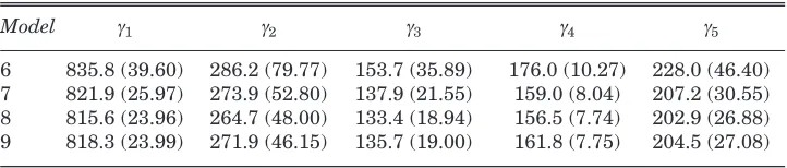
Continuing to the γparameters, estimates are shown in Table 2.
Table 2: Estimates of γParameters with Standard Errors
Model γ1 γ2 γ3 γ4 γ5
6 835.8 (39.60) 286.2 (79.77) 153.7 (35.89) 176.0 (10.27) 228.0 (46.40) 7 821.9 (25.97) 273.9 (52.80) 137.9 (21.55) 159.0 (8.04) 207.2 (30.55) 8 815.6 (23.96) 264.7 (48.00) 133.4 (18.94) 156.5 (7.74) 202.9 (26.88) 9 818.3 (23.99) 271.9 (46.15) 135.7 (19.00) 161.8 (7.75) 204.5 (27.08)
Again differences are small with almost all estimates across models (7), (8) and (9) equal to two significant digits. For model 6 – the LES in expenditure form – estimates do seem slightly larger than for the other three models, but the magnitudes make no practical difference. For example, the own-price elasticity9of food (at the 1999 end-point) calculated from model 6 is –.44 and
calculated from model 9 it is –.45. For standard errors the dominating difference is between model (6), where standard errors do seem larger and models (7), (8) and (9), within which differences are not appreciable. This contradicts the idea that the issue of bounds and multinormality can matter
9The formula being –1 + γ
[image:7.498.66.427.379.456.2]much, because (7) is at least as suspect as (6) in that regard. Probably the data conditioning by scaling, involved in all models except (6), is responsible.
IV CONCLUDING REMARKS
As we have already indicated, we do agree with Fry et al.,(1996) that a theoretical case can be made for logistic transformation of shares and, in particular, for estimating the LES in the form (9), when we are confident of the utility maximisation context. While we did find it intuitively plausible that estimates of parameters should be affected by the treatment of the stochastic terms, the actual magnitudes of differences between parameter estimates and standard errors just do not appear to be of appreciable practical importance. But if this is disappointing in terms of return to increased sophistication of analysis, it is reassuring about the reliability of past applied research findings based on the LES, at least where annual time series data on broad commodities aggregated over households were employed.
Even so, should (9) always be estimated on the grounds that it is still the theoretically preferred model? Perhaps, but not on its own though, partly because good starting estimates are needed to work with (9) for the reasons given in the previous section. There is also the possibility that the solution is not compatible with utility maximisation. If some true βi are negative, or if
estimated γ are large relative to y, iterative solution of (9) could become meaningless. So it would seem (7), taking account of the possibly less precise estimates of the γi by (6), ought to be solved as a preliminary to (9). For our
data the “preliminary” would be virtually identical to the “final”, but perhaps that might not be always so.
The assumptions implicit in the LES are restrictive which was why our analysis was limited to broad commodity categories of non-durable goods. Could the finding that the stochastic specification did not matter much extend to other, more behaviourally flexible, models? The complicating issue is that, as discussed in Section I, many models currently popular for demand analysis are not globally regular in their deterministic components. So the objective of dependent variable transformation would be as much or more about improving the plausibility of the deterministic term as about appropriateness of the stochastic formulation. Perhaps the findings suggest that if a model can be reformulated so that its deterministic component is regular then the specification of the stochastic component is comparatively unimportant when analysing national level data.
households to national level. However, demand equations and sometimes complete systems are often estimated using microdata from household level surveys and with much more finely differentiated commodities. It is probably always true that much greater variation in commodity consumptions exist at household or individual levels, with correspondingly greater variances of distributions. So stochastic specification may matter much more in microlevel applications as, indeed, Fry et al., remarked. However, it is obvious that in these circumstances the LES would not have been employed to start with, because its implicit assumptions are then implausible, and because extra explanatory variables (demographic, for example) besides prices and income may be required to model microdata.10The findings in this paper probably do
not have much evidential value for model choice when analysing microdata.
REFERENCES
BARNETT, W. A., 1983. “New Indices of Money Supply and the Flexible Laurent Demand System”, Journal of Business and Economic Statistics, Vol. 1, pp. 7-23. BARNETT, W. A. and Y. W. LEE, 1985. “The Global Properties of the Minflex Laurent,
Generalised Leontief and Translog Functional Forms”, Econometrica, Vol. 53, pp. 1421-1438.
BOYLE, G. E. 1996. “A MAIDS Model of Irish Meat Demand”,The Economic and Social Review,Vol. 27, No. 4, pp, 309-319.
CASEY, M. G., 1973. “An Application of the Samuelson-Stone Linear Expenditure System to Food Consumption in Ireland”, The Economic and Social Review,Vol. 4, No. 3, pp. 309-342.
CHALFANT, J. A., 1987. “A Globally Flexible, Almost Ideal Demand System”, Journal of Business and Economic Statistics, Vol. 5, pp. 233-242.
CONNIFFE, D., 1993. “Logistic Transformation of the Budget Share in Engel Curves and Demand Functions”, The Economic and Social Review, Vol. 25, No. 1, pp. 49-56.
COOPER, R. J. and K. R. McLAREN, 1992. “An Empirically Oriented Demand System with Improved Regularity Properties”, Canadian Journal of Economics, Vol. 25, pp. 653-668.
DEATON, A. and J. MUELLBAUER, 1980. “An Almost Ideal Demand System”,
American Economic Review, Vol. 70, pp. 312-316.
DUFFY, D., J. FITZ GERALD, I. KEARNEY, J. HORE and C. MACCOILLE, 2001.
Medium-Term Review 2001-2007, Dublin: The Economic and Social Research Institute.
10Indeed the dependent variables may change too. If considering substantial durable goods, or
FRY, J. M., T. R. L. FRY and K. R. McLAREN, 1996. “The Stochastic Specification of Demand Share Equations: Restricting Budget Shares to the Unit Simplex”,
Journal of Econometrics, Vol. 73, pp. 377- 385.
HOUTHAKKER, H. S., 1960. “Additive Preferences”, Econometrica, Vol. 28, pp. 244-256.
LESER, C. E. V., 1963. “Forms of Engel Functions”,Econometrica, Vol. 31, pp. 694-703. MCCARTHY, C., 1977. “Estimates of a System of Demand Equations using Alternative Commodity Classifications of Irish Data, 1953-1974”, The Economic and Social Review,Vol. 8, No. 3, pp. 201-211.
O’RIORDAN, W., 1976. “Consumer Response to Price and Income Change”, Journal of the Statistical and Social Inquiry Society of Ireland, Vol. 23, pp. 65-89.
SHAZAM, 2001. User’s Reference Manual Version 9.0, Vancouver: Northwest Econometrics.