Abstract—In this paper, based on the space fractional order diffusion equation, we estimate the equation parameters by using an improved ant colony algorithm, that is, the Niche Ant Colony Algorithm (NACA) based on fitness sharing principle. Its efficiency is verified by application of 20 standard test functions of 1–20 variables compared with standard ant colony algorithm and standard genetic algorithm. Then, the parameters identification of the space fractional order diffusion equation is performed with the niche ant colony algorithm. Furthermore, the sensitivity analysis of the proposed method to transition probability and pheromone evaporation factor has been studied. The numerical results indicate that NACA has rapid convergent speed, high calculation precision, and good anti-noise property.
Index Terms—space fractional order diffusion equation, parameter identification, niche ant colony algorithm, fitness sharing principle
I. INTRODUCTION
T is well known that the classical diffusion equations have played many important roles in modeling contaminant diffusion processes. However, in the recent two decades, people realized that the classical model is inadequate to simulate many real situations, where a particle plume spreads faster or slower than predicted by the integer-order diffusion equation, and shifted their partial focus to fractional order diffusion equations. Some fractional order diffusion equations are proved to be successfully used for modeling some anomalous diffusion physical phenomena in many fields, such as environment engineering, chemical engineering, automatic control, and so on.
In recent years, with the further developments of fractional order differential equations in the applied sciences, there exist several pieces of research on theoretical analysis and numerical methods for the forward problem of space fractional order diffusion equations. Ma [1] studied the framework and convergence analysis of finite element method
Manuscript received September 25, 2016; revised January 19, 2017.This work was supported by the National Science Foundation of China (Grant No. 41004052), and supported by the Specialized Research Fund for the Doctoral Program of Higher Education of China (Grant No. 20102302120072).
Xinming Zhang (corresponding author) is withthe College of Science of Harbin Institute of Technology Shenzhen Graduate School, Shenzhen, Guangdong, 518055 PR China, e-mail: [email protected].
Di Yuan is with the Department of Applied Mathematics of Harbin Institute of Technology Shenzhen Graduate School, Shenzhen, Guangdong,
for space fractional order differential equations with inhomogeneous boundary conditions. Sakamoto and Yamamoto [2] showed some better results on the uniqueness and stability of the solution to the initial value/boundary value problems for fractional diffusion-wave equations. Huang et al. [3] proposed a high order finite difference-spectral method for solving space fractional diffusion equations by combining the second order finite difference method in time and the spectral Galerkin method in space. Chen and Deng [4] derived a class of fourth order approximations for space fractional derivatives and used the derived schemes to solve the space fractional order diffusion equation with variable coefficients in one-dimensional and two-dimensional cases. Japundžić and Rajter-Ćirić [5] considered a space fractional reaction-advection-diffusion equation which is actually a semi-linear Cauchy problem with a spatial fractional order derivative operator and proved assertions concerning the existence and uniqueness of solution within certain Colombeau space. Yang, Liu, and Turner [6] considered the numerical solution of two types of fractional partial differential equation with Riesz space fractional derivatives (FPDE-RSFD) on a finite domain and obtained some better results. A.Bouhassoun [7] used telescoping decomposition method to derive approximate analytical solutions of fractional differential equations and provided a simple way to adjust and control the convergence region of solution series by introducing the multistage strategy. M.Asgari [8] proposed a new numerical method for solving a linear system of fractional integro-differential equations based on the new operational matrices of triangular functions. H. Song et al.[9] investigated numerical solutions of generalized variable order fractional partial differential equations by using Bernstein polynomials. Meanwhile, there are some researches for inverse problems of fractional differential equations. For a backward problem of the time-fractional diffusion equation, Liu and Yamamoto [10] proposed a regularizing scheme by the quasi-reversibility with fully theoretical analysis and tested its numerical performance. Zheng and Wei [11] studied a backward diffusion problem for a space fractional diffusion equation in a strip domain by the Fourier regularization method. Under an assumption that the unknown source term is time independent, Zhang and Xu [12] deduced the analytical solution based on the method of the eigenfunction expansion for an inverse source problem of a fractional diffusion equation and proved the uniqueness of the inverse problem by analytic continuation and Laplace transform. Rodrigues et al. [13] dealt with the use of the conjugate gradient method in
A Niche Ant Colony Algorithm for Parameter
Identification of Space Fractional Order
Diffusion Equation
Xinming Zhang and Di Yuan
I
IAENG International Journal of Applied Mathematics, 47:2, IJAM_47_2_11
conjunction with an adjoint problem formulation for the simultaneous estimation of the spatially varying diffusion coefficient and of the source term distribution in a one-dimensional nonlinear diffusion problem. Cheng et al. [14] proved the uniqueness in the inversion problem of simultaneously determining a fractional order and a space-dependent diffusion coefficient of a one-dimensional fractional diffusion equation with zero Neumann boundary conditions and the additional boundary data. Bondarenko and Ivaschenko [15] constructed a weighted difference scheme which is conditionally stable and convergent with zero Dirichlet boundary conditions to solve the forward problems of time fractional diffusion equation and presented numerical results by using the Levenberg–Marquart algorithm. However, most of the results from these studies have been obtained by using the traditional deterministic optimization methods. The stochastic global optimization methods to estimate the parameters in the inverse problems of fractional differential equations have rarely been reported. In fact, compared with the deterministic optimization methods, stochastic optimization methods require no prior assumptions or transformation of the objective function and have been widely applied to the parameters identification of the other research fields [16-18]. In this article, we will consider the inversion problem for determining the space fractional order and source term of fractional order diffusion equation with the niche ant colony algorithm. To our knowledge, no relevant report is yet available in the field of the previous inversion problem with the niche ant colony algorithm. As a newly developed global optimal method, ant colony algorithm has also captured the interest of numerous scholars. The original ant colony algorithm was proposed by Colorni et al. [19] in the 1990s. This algorithm is an optimization methodology based on the foraging behavior of Argentine ants. In 1995, Bilchev [20] proposed the continuous ant colony algorithm for the first time, however, what they investigated actually was the genetic algorithm based on the ant colony algorithm. Li [21] proposed an adaptive ant colony system algorithm for continuous-space optimization problems. Chen et al. [22] presented a continual domain ant colony algorithm based on overlapping mutation operations. Dreo [23-24] proposed a continuously interacting ant colony algorithm based on an intensive non-hierarchical process. Chen [25] proposed a method that approximates the variance of continuous functions with discrete points. Zhang [26] proposed a continual domain ant colony algorithm for constrained multiobjective function optimization. In general, for ant colony algorithm, however, the information difference is achieved through genetic manipulation, which easily causes premature events. To address the premature defect, various niche approaches, usually called niche techniques, were recently developed. Among these niche methods (including crowding [27], fitness sharing [28], clearing [29], and clustering-based niche methods [30]), fitness sharing is a well-known niche technique that offers a variety of modified schemes [31-33]. Niche, as an evolutionary computation concept, was first formally applied to genetic algorithm [34]. However, niche has also been applied to other algorithms, such as the ant colony algorithm, and some promising results have been obtained [35-36]. Although NACA has been
adopted to deal with a number of optimization problems, no relevant report is yet available in the field of parameter inversion. In this paper, NACA based on the fitness-sharing principle is applied to the parameters inversion of the space fractional order diffusion equation and provides some improved results.
The remainder of work is organized as follows: the niche ant colony algorithm (NACA) based on fitness sharing principle is introduced in detail in Section 2. Section 3 gives several numerical results of multimodal function optimization. Section 4 shows several inversion examples of the parameter identification of the space fractional order diffusion equation. Finally, the conclusion is presented in the final section.
II. NICHE ANT COLONY ALGORITHM
The concept of niche method comes from the analogy with natural ecosystems, which are often composed by different subspaces (niches) that support different types of life (species or organisms). Within a niche, the available resources are finite and must be shared among its individuals. On the other hand, among different niches, there will be no conflict for the resources. In evolutionary computation, a niche is commonly referred to as an optimum of the domain, and the fitness represents the resources of that niche. Niche technique can promote the diversity of a population, and improve the capability of individuals in exploration.
A. NACA Based on Fitness Sharing Principle
Niche formation, specifically relative to fitness sharing, was explained by Goldberg and Richardson [28] with a variation of the k-armed bandit problem. The niche algorithm was applied to find and preserve multiple solutions in genetic algorithm. With the fitness-sharing approach, the search landscape is modified by reducing the payoff in densely populated regions. This approach reduces the fitness of an individual by an amount that is proportional to the number of similar individuals in the population. On the basis of the same theory, we apply the fitness-sharing algorithm to ACA and propose the NACA based on fitness sharing principle.
Similarly, in this paper, a sharing function is defined to calculate the niche counts, which are further used immediately prior to the selection operation to de-rate the fitness of individuals in densely populated subspaces as follows:
1 ( )
0
ij
ij ij
d
d Sh d
otherwise
(1)
where is the niche radius that is given by the formula:
2 1
(1 / (2n )) n ( u l) k k k
q x x
(2)where q is the number of niches,
n
is the dimension of the feasible region, { , }u lk k
x x denote the upper and lower bounds of the kth dimension of the feasible region, dij is the distance
between individualsi andj, andi j, 1, 2,...,N, N denotes the population size. The sharing function describes the similarity among different individuals: Sh d( ij) 1 indicates
that i and j are the same individuals or dij 0, whereas
IAENG International Journal of Applied Mathematics, 47:2, IJAM_47_2_11
( ij) 0
Sh d suggests that i and j belong to different niches. In (1), is a constant (typically set to one) used to control the shape of the sharing function. The similarity among individuals for real coded evolutionary algorithms is computed through the Euclidean distance in real-valued space.
For each individual i, some individuals are measured to be similar by . The raw fitness fi (the objective function
value for the individual i ) is to be shared with such individuals. The niche count mi is given by:
1
Sh
N
i ij
j
m d
(3)The value of mi is comparable to the number of
individuals around the ith individual. A large value indicates that more individuals surround the ith individual. The shared fitness of individual i, with raw fitness fi, is given by:
i i
i f f
m
(4) Through fitness sharing, the replicas and the offspring of an individual are produced inversely proportional to the similar ones in the same niche. Even elitists could not take over the population, which means that the fitness-sharing scheme is capable of counterbalancing the genetic drift. Thus, the fitness-sharing technique allows the exploration and exploitation of fitness landscape by favoring the formation of stable subpopulations. With properly parameterized fitness sharing (population size N and niche radius ), the niche equilibrium is eventually reached, where all individuals are distributed among niches according to their fitness, and all species of the identified niches are maintained to the final population.
A general pseudocode representation is provided as follows:
Algorithm: Niche Ant Colony Algorithm based on the
Fitness Sharing Principle
Procedure Initialization
(i) Parameters Initialization: such as population size, the
global transition probability, the evaporation coefficient of pheromone, the proportional factor, the feasible region, and the radius of niche (Obtained from (2) );
(ii) Population Initialization: for i1 to psize do
*1
X i start end start rand ; (The initial position of ants)
FitnessValue i
k f X i
; (The fitness value before sharing, where f is the optimization function)end for end procedure
* The function rand
1 provides samples from the uniform[0,1] distribution.
while stopping criterion not met do
De-rate quality;
Calculate transition probability;
Update positions of ants (in the feasible region);
Update pheromones;
end while
Procedure De-rate quality
for i1 to do NicheCount0
for j1 to do
ddistance
p pi, j
if d thenShareValue
1 d
elseShareValue 0 endif
NicheCountNicheCount ShareValue
end for
/
FitnessValue Modified FitnessValue NicheCount (The fitness value after sharing)
end for end procedure
Procedure Calculate transition probability
[i] k/
T FitnessValue Modified ; (The initial pheromone)
_ (T)
T BestMax
For i1 to psize do
Prob i[ ] ( _ T Best T T Best ) / _ end for
For i1 to psize do
if Prob i[ ]P0
TempX i
min step_ *
rand
1 0.5
elseTempX i
max_step*
rand
1 0.5
endififT mpe start
T mpe start
elseif Temp end Temp end endif
end for end procedure
Procedure Update positions of ants and pheromones
For i1 to psize do
if
Temp
/NicheCount f X i
/NicheCount
X i Temp
/FitnessValue Modified f X i NicheCount _ 1 ec * /
T i new p T i k f X i (Update pheromones) endif
end for end procedure
IAENG International Journal of Applied Mathematics, 47:2, IJAM_47_2_11
The description of the NACA can also be given in Figure 1.
Fig. 1. Flowchart of NACA.
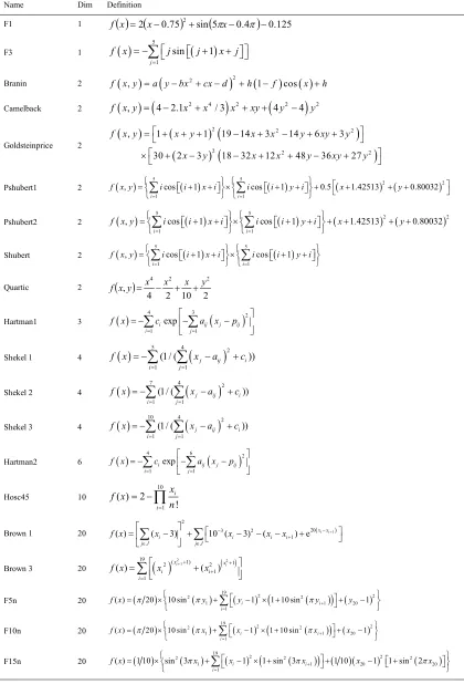
III. APPLICATION IN MULTIMODAL FUNCTION OPTIMIZATION It is well known that multimodal function optimization is useful for analyzing algorithm properties. In this section, in order to test the performance of NACA based on fitness sharing principle, NACA is applied to find the global optimum of 20 nonlinear test functions. The benchmark functions are described in Table I and the properties of these
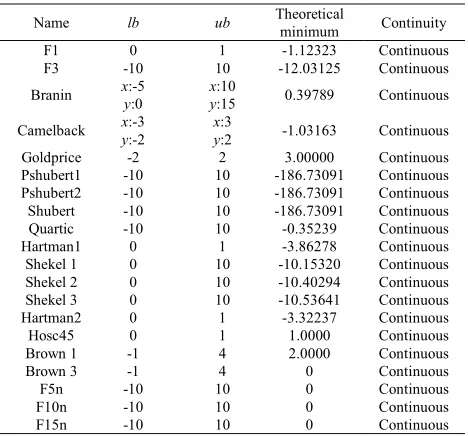
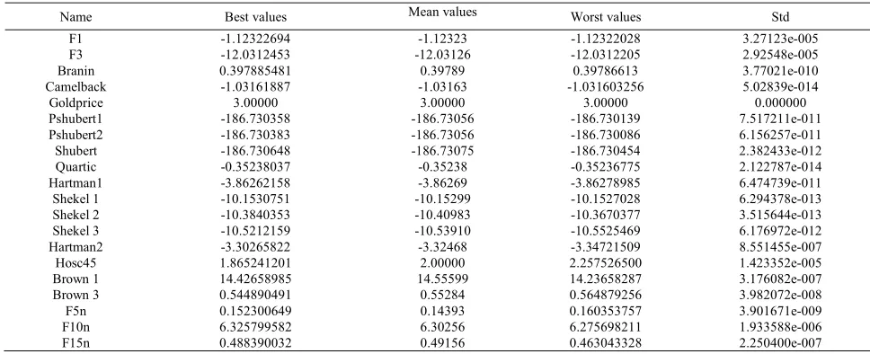
[image:4.612.311.545.502.720.2]benchmark functions are given in Table II. More details about these test functions can be found in the literature [37]. The aim of this study is the search for global optimum of nonlinear functions. So it is very important that our NACA effectively converges to this optimum. The global optimization of the 20 test functions is accomplished by use of the following methods: standard binary-coded genetic algorithm (Named SGA [37]), standard ant colony algorithm (Named ACA) and niche ant colony algorithm (Named NACA). As we all known, the metaheuristic methods are generally based on random distribution. In order to remove the influence of the randomness, 50 runs are carried out to obtain an average result. Setting the number of niches to 10, the number of individuals is 100, the transition probability is 0.7, the pheromone evaporation factor is 0.2, and the radius is calculated according to (2). The maximum iteration is 200. All algorithms have been tested in MATLAB (version 7.1) with double precision over the same Pentium IV personal computer with a 2.3GHz processor, running Windows 7 operating system over 2G of memory. The computational results and calculating accuracy of the 20 nonlinear test functions on global optimization with the methods of SGA, ACA and NACA are given in Table III. Table IV gives the results of statistical tests, including average, best, worst performance, and Std. From Table III and Table IV, we can conclude that for the 20 test functions, the results achieved with NACA are satisfactory in global optimum. Moreover, by carefully looking at the Table III, we can see, the obtained results indicate that incorporating niche technique in the ACA would lead to a significant increase in the performance of ACA. It is apparent that when the niche technique is taken into account, the performance is improved as compared to the other methods. This verifies the effectiveness and the ability of the proposed NACA in solving the global numerical optimization problem.
TABLE II Properties of the benchmark functions (lb denotes lower bound, ub denotes upper bound ) Name lb ub Theoretical minimum Continuity
F1 0 1 -1.12323 Continuous F3 -10 10 -12.03125 Continuous Branin xy:-5 :0 xy:10 :15 0.39789 Continuous Camelback xy:-3 :-2 xy:3 :2 -1.03163 Continuous Goldprice -2 2 3.00000 Continuous Pshubert1 -10 10 -186.73091 Continuous Pshubert2 -10 10 -186.73091 Continuous Shubert -10 10 -186.73091 Continuous Quartic -10 10 -0.35239 Continuous Hartman1 0 1 -3.86278 Continuous Shekel 1 0 10 -10.15320 Continuous Shekel 2 0 10 -10.40294 Continuous Shekel 3 0 10 -10.53641 Continuous Hartman2 0 1 -3.32237 Continuous Hosc45 0 1 1.0000 Continuous Brown 1 -1 4 2.0000 Continuous
Brown 3 -1 4 0 Continuous
F5n -10 10 0 Continuous
F10n -10 10 0 Continuous
F15n -10 10 0 Continuous
Yes
No Start
Initialize parameter and population
De-rate quality
Calculate transition probability
Update positions of ants (in the feasible region)
Update pheromones
Is termination condition
met?
End Output the best
IAENG International Journal of Applied Mathematics, 47:2, IJAM_47_2_11
TABLE I Benchmark functions Name Dim Definition
F1 1 f
x 2x0.75
2sin
5x0.4
0.125F3 1
5
1
sin 1
j
f x j j x j
Branin 2 f x y
,
a y bx
2cx d
2h
1 f
cos
x hCamelback 2 f x y
,
4 2.1 x2x4/ 3
x2xy
4y24
y2Goldsteinprice 2
2 2 2
2 2 2
, 1 1 19 14 3 14 6 3
30 2 3 18 32 12 48 36 27
f x y x y x x y xy y
x y x x y xy y
Pshubert1 2
5 5
2 2
1 1
, cos 1 cos 1 0.5 1.42513 0.80032
i i
f x y i i x i i i y i x y
Pshubert2 2
5 5
2 2
1 1
, cos 1 cos 1 1.42513 0.80032
i i
f x y i i x i i i y i x y
Shubert 2
5 5
1 1
, cos 1 cos 1
i i
f x y i i x i i i y i
Quartic 2
2 10 2 4 , 2 2
4 x x y
x y x
f
Hartman1 3
4 3 2
1 1
exp
i ij j ij
i j
f x c a x p
Shekel 1 4
5 4 2
1 1
(1/ ( j ij i))
i j
f x x a c
Shekel 2 4
7 4 2
1 1
(1/ ( j ij i))
i j
f x x a c
Shekel 3 4
10 4 2
1 1
(1/ ( j ij i))
i j
f x x a c
Hartman2 6
4 6 2
1 1
exp
i ij j ij
i j
f x c a x p
Hosc45 10
10
1
( ) 2 ! i i x f x n
Brown 1 20 1
2
20
3 2
1
( ) ( 3) 10 ( 3) ( ) e x xi i
i i i i
j J j J
f x x x x x
Brown 3 20
2 2
1
19 ( 1) 1
2 2
1 1
( ) xi ( )xi
i i
i
f x x x
F5n 20
19
2 2
2 2
1 1 20
1
( ) 20 10 sin i 1 1 10 sin i 1
i
f x y y y y
F10n 20 2 19 2
2
21 1 20
1
( ) 20 10 sin i 1 1 10 sin i 1
i
f x x x x x
F15n 20
19
2 2
2 2 2
1 1 20 20
1
( ) 1 10 sin 3 i 1 1 sin 3 i 1 10 1 1 sin 2
i
f x x x x x x
IAENG International Journal of Applied Mathematics, 47:2, IJAM_47_2_11
TABLE III Mean Results with SGA, ACA, and NACA
Name Theoretical minimum Minimum found with SGA Absolute error Minimum found with ACA Absolute error Minimum found with NACA Absolute error
F1 -1.12323 -1.12323 0 -1.12384 -0.00061 -1.12323 0
F3 -12.03125 -12.03120 5e-05 -12.03673 -0.00548 -12.03126 -1e-05
Branin 0.39789 0.39798 9e-05 0.39773 -0.00016 0.39789 0
Camelback -1.03163 -1.03163 0 -1.03412 -0.00249 -1.03163 0
Goldprice 3.00000 3.00000 0 3.00842 0.00842 3.00000 0
Pshubert1 -186.73091 -186.73000 0.00091 -186.73903 -0.00812 -186.73056 0.00035 Pshubert2 -186.73091 -186.73100 -9e-05 -186.73146 -0.00055 -186.73056 0.00035 Shubert -186.73091 -186.73100 -9e-05 -186.73625 -0.00534 -186.73075 0.00016 Quartic -0.35239 -0.35239 0 -0.35689 -0.0045 -0.35238 1e-05 Hartman1 -3.86278 -3.86249 0.00029 -3.86731 -0.00453 -3.86269 9e-05 Shekel 1 -10.15320 -10.13490 0.0183 -10.15589 -0.00269 -10.15299 0.00021 Shekel 2 -10.40294 -10.16770 0.23524 -10.39041 0.01253 -10.40983 -0.00689 Shekel 3 -10.53641 -10.40340 0.13301 -10.53003 0.00638 -10.53910 -0.00269 Hartman2 -3.32237 -3.30652 0.01585 -3.32644 -0.00407 -3.32468 -0.00231
Hosc45 1.0000 1.99506 0.99506 2.00000 1 2.00000 1
Brown 1 2.0000 43.62810 41.6281 23.63478 21.63478 14.55599 12.55599
Brown 3 0 1.30600 1.306 1.74537 1.74537 0.55284 0.55284
F5n 0 0.47353 0.47353 0.75752 0.75752 0.14393 0.14393
F10n 0 7.83515 7.83515 28.47829 28.47829 6.30256 6.30256
[image:6.612.67.545.96.296.2]F15n 0 0.52117 0.52117 36.82356 36.82356 0.49156 0.49156
TABLE IV The final values of NACA for benchmark functions
Name Best values Mean values Worst values Std
F1 -1.12322694 -1.12323 -1.12322028 3.27123e-005
F3 -12.0312453 -12.03126 -12.0312205 2.92548e-005
Branin 0.397885481 0.39789 0.39786613 3.77021e-010
Camelback -1.03161887 -1.03163 -1.031603256 5.02839e-014
Goldprice 3.00000 3.00000 3.00000 0.000000
Pshubert1 -186.730358 -186.73056 -186.730139 7.517211e-011
Pshubert2 -186.730383 -186.73056 -186.730086 6.156257e-011
Shubert -186.730648 -186.73075 -186.730454 2.382433e-012
Quartic -0.35238037 -0.35238 -0.35236775 2.122787e-014
Hartman1 -3.86262158 -3.86269 -3.86278985 6.474739e-011
Shekel 1 -10.1530751 -10.15299 -10.1527028 6.294378e-013
Shekel 2 -10.3840353 -10.40983 -10.3670377 3.515644e-013
Shekel 3 -10.5212159 -10.53910 -10.5525469 6.176972e-012
Hartman2 -3.30265822 -3.32468 -3.34721509 8.551455e-007
Hosc45 1.865241201 2.00000 2.257526500 1.423352e-005
Brown 1 14.42658985 14.55599 14.23658287 3.176082e-007
Brown 3 0.544890491 0.55284 0.564879256 3.982072e-008
F5n 0.152300649 0.14393 0.160353757 3.901671e-009
F10n 6.325799582 6.30256 6.275698211 1.933588e-006
F15n 0.488390032 0.49156 0.463043328 2.250400e-007
We have also performed a comparison of NACA with six other methods of iterative improvement listed in Table V: pure random search (PRS) [38], multistart (MS) [39], simulated diffusion (SD) [40], simulated annealing (SA) [41], tabu search (TS) [42], and standard binary-coded genetic algorithm (SGA) [37]. The efficiency is qualitative in terms of the number of function evaluations necessary to find the global optimum. Each program is stopped as soon as the relative error between the best point found and the known global optimum is less than 1%. The numbers of function evaluations used by the various algorithms to optimize four test functions are listed in Table VI. It is noted that we do not program ourselves the competitive algorithms used for the comparison, but we report the results published by Cvijovic
and Klinowski [42] and Andre et al. [37]. We can see that results achieved with NACA are satisfactory in global optimum and convergent speed (see the numbers of function evaluations in Table VI). In addition our results are the average outcome of 50 independent runs.
TABLE V Global optimization methods used for performance analysis
Method Name Reference
PRS Pure random search 38
MS Multistart 39
SD Simulated diffusion 40
SA Simulated annealing 41
TS Tabu search 42
SGA Standard binary-code genetic algorithm 37
NACA This work
IAENG International Journal of Applied Mathematics, 47:2, IJAM_47_2_11
[image:6.612.62.546.333.530.2]TABLE VI Number of function evaluations in global optimization of test functions by the seven different methods
Method Function Goldprice Branin Hartman 1 Hartman2
PRS 5125 4850 5280 18090
MS 4400 1600 2500 6000
SD 5439 2700 3416 3975
SA 563 505 1459 4648
TS 486 492 508 2845
GA 4632 2040 1680 53792
NACA 427 389 408 932
IV. PARAMETER INVERSION BASED ON THE SPACE FRACTIONAL DIFFUSION EQUATION A. Example 1 - Inversion for Fractional Order
A space fractional order advection-diffusion equation is given as follows:
0
( , ) ( , ) ( , )
( ) ( ) ( , ),0 , 0
( ,0) ,0
(0, ) , 0
( , ) L, 0
C x t C x t C x t
a x b x q x t x L t
t x x
C x C x x L
C t C t
C L t C t
(5) where C is the mean concentration of substance dispersed in the general cross section of the flow,
0,1 ,
1, 2 are called the fractional orders of the derivative in space, a x( )is the advection coefficient and b x( ) is the diffusion coefficient, q x t
, is the source. C x t( , ), C x t( , )x x
here
mean the Riemann-Liouville derivatives:
0 2
1 0
( , ) 1 ( , )
, 0 1
(1 ) ( )
( , ) 1 ( , )
,1 2
(2 ) ( )
x
x
C x t C t
d x
x x
C x t C t
d x x x
(6)
where
is Gamma function.Suppose the distributions of C x t
, in x x 0, 0x0 Lor in t T are known, an inverse problem of fraction order identification for convection–diffusion equation is making certain fractional orders , . Having available an auxiliary measurement of the concentration C x t
, in a point set downstream of the source and the time behavior of the concentration at the domain boundaries, we wish to decide the fractional orders , .In this paper, if we let ( ) (3 ) (3 )
a x x
, 2 ( ) (3 )
b x x
,
2
C x x ,
0 0
C , 42 1
L
C t ,
2 2 2 2 1
( , ) (4 1)( ) 4(2 )
q x t t x x x t , then one
can get the solution of (5) as follows:
2 2
( , ) (4 1)
C x t t x
(7) In order to decide the fractional orders , , some
conditions should be given. In this paper, we give the additional condition C x T
,
for T1. From (7), we can see that C x T
,
depends on , . So, the identification problem of fractional orders , can be formalized as follows:
, ,
1
min n obs j , cal j ,
j
f C C
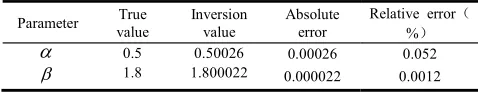
(8) where Cobs j, is observed value, and Ccal j, is calculated value. This is a complicated nonlinear parameter optimization problem. This kind of parameter optimization model is very intractable mathematically with traditional optimization methods. We use NACA to solve it in this paper. We initially perform the inversion of two parameters without noise. The different inversion parameter intervals are as follows:0.1 0.8 , 1.5 2.0. Setting the number of niches to 4, the number of individuals is 100, the transition probability is 0.7, the pheromone evaporation factor is 0.2, the maximum iterations is 200, and the radius is still calculated according to (2). Similar to that in Section 3, 50 runs are carried out to obtain an average result in the following simulations. Table VII shows the inversion results. As we have seen, the inversion precisions of these parameters are high and the relative errors of the parameters inversion can be maintained at less than 0.05%. The CPU time of two-parameter inversion is 2.38s.
In order to show the superiority of NACA, the other two optimization methods (ant colony algorithm (ACA) and standard genetic algorithm (SGA)) are used to inverse the fractional order. Each algorithm is statistically compared with NACA by a statistical test called t-test for independent samples with significance level of 0.05. The real number 1 denotes that the NACA algorithm is superior to or inferior to other algorithms. For each problem, the algorithms carry out 50 independent runs. The setting of the NACA parameters is the same as the previous cases. For SGA, the crossover rate is 0.8, and the mutation rate increases linearly from 0.001 to 0.6 during the evolution. For ACA the transition probability is 0.7, the pheromone evaporation factor is 0.2, the maximum iterations is 200. The iterative process of the objective function is shown in Fig.2.The results on the parameter inversion problems (Mean, Best, Worst, Std, and t-test results) are recorded in Table VIII. It can be seen that NACA produces superior performance than ACA and SGA in terms of average, best, and worst performance. Furthermore, the Std of CS is much smaller than these two methods. In summary, NACA outperforms other algorithms in statistically significant fashion over the parameter estimation problems and has a relatively high possibility of finding the satisfactory inverse results.
TABLE VII The parameter inversion results without noise Parameter value True Inversion value Absolute error Relative error(
%) 0.5 0.50026 0.00026 0.052 1.8 1.800022 0.000022 0.0012
IAENG International Journal of Applied Mathematics, 47:2, IJAM_47_2_11
[image:7.612.306.545.677.723.2]TABLE VIII The inversion results for parameter inversion problem
Algorithm
Best Mean Worst Std p-value Best Mean Worst Std p-value ACA 0.50098 0.50145 0.50223 2.467e-2 2.26e-18 (1) 1.80095 1.80164 1.80621 4.852e-2 2.84e-19 (1)
[image:8.612.65.547.172.265.2]SGA 0.51023 0.52238 0.54827 6.253e-1 1.68e-21 (1) 1.81021 1.830592 1.87264 8.124e-1 5.38e-22 (1) NACA 0.50018 0.50026 0.50035 1.239e-4 1.800012 1.800022 1.800030 5.268e-5
TABLE IX The inversion results with different transition probabilities
Transition probability Relative error (%) Relative error (%) Time (s)
0.1 0.52107 4.214 1.850369 2.798 2.26237
0.2 0.51295 2.590 1.808491 0.472 2.63212
0.3 0.49056 1.888 1.782167 0.991 2.77263
0.4 0.53061 6.122 1.762010 2.111 2.33598
0.5 0.50821 1.642 1.830065 1.670 2.47244
0.6 0.50469 0.938 1.818503 1.028 2.59590
0.7 0.50026 0.052 1.800022 0.001 2.38249
0.8 0.50191 0.382 1.790042 0.553 2.67292
[image:8.612.72.545.291.391.2]0.9 0.47903 4.193 1.859105 3.284 2.71289
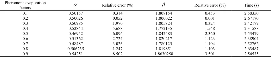
TABLE X The inversion results with different pheromone evaporation factors Pheromone evaporation
factors Relative error (%) Relative error (%) Time (s)
0.1 0.50157 0.314 1.808154 0.453 2.50350
0.2 0.50026 0.052 1.800022 0.001 2.67170
0.3 0.50985 1.970 1.805824 0.324 2.42177
0.4 0.52844 5.688 1.772135 1.548 2.31588
0.5 0.46952 6.096 1.842483 2.360 2.53479
0.6 0.51362 2.724 1.820217 1.123 2.38904
0.7 0.48487 3.026 1.780125 1.104 2.52762
0.8 0.506235 1.247 1.819851 1.103 2.63487
0.9 0.54251 8.502 1.8630258 3.501 2.54535
Fig. 2. Convergence of objective function.
(a) Influences of algorithm parameters
In this subsection, the influences of algorithm parameters to inversion results are discussed, including the transition probability and the pheromone evaporation factor. The setting of parameters is the same as the previous example. Table IX and Table X show the inversed results of fractional order with different algorithm parameters. As shown in Table IX, the optimal results go to be the best when the transition probability reaches 0.7, while the CPU time has no evident
change. From the obtained inversed results in Table X, it is indicated that when pheromone evaporation factor equals to 0.2, the inversion procedure finds the optimal results. And, as a consequence, we have used these two values for all the previous parameters inversion.
(b) Anti-noise property
To test the robustness and stability of NACA, we will add different levels of noise to the seismograms as follows:
*
, ,
1
obs j obs j
C
C
(9)
where is the noise level; * ,
obs j
C is the measured velocity with noise;
is the random number according to standard normal distribution. In this process, the parameter values are the same as the foregoing example. Tables XI-XIII show the inversion results with 5%, 10% and 15% noises, respectively. The tables show that the inversion results are satisfactory.TABLE XI The parameter inversion results with 5% noise Parameter value True Inversion value Absolute error Relative error (%)
0.5 0.500324 0.000324 0.0684 1.8 1.799347 0.000653 0.0363
TABLE XII The parameter inversion results with 10% noise Parameter value True Inversion value Absolute error Relative error (%)
0.5 0.499345 0.000655 0.1310 1.8 1.801405 0.001405 0.0781
IAENG International Journal of Applied Mathematics, 47:2, IJAM_47_2_11
[image:8.612.75.294.415.599.2] [image:8.612.308.546.631.673.2] [image:8.612.307.547.697.741.2]TABLE XIII The parameter inversion results with 15% noise Parameter value True Inversion value Absolute error Relative error (%)
0.5 0.498851 0.001149 0.2298 1.8 1.804751 0.004751 0.2639
B. Example 2 - Inversion for Source Term
In this subsection, we will inverse the source term of the following space fractional order diffusion equation initial-boundary value problem with NACA.
( ) ( , ),1 2, 0, 0
u u
d x q x t t x l
t x
(10)
0 1 2
( , 0) ( ) (0, ) ( ) ( , ) ( ) u x f x u t b t u l t b t
(11)
where f0
x is an initial function, b t1
and b t2
areboundary functions, d x( ) is the diffusion coefficient, q x t , is the source term.
(a) The implicit difference scheme for forward problem
Firstly let us deal with numerical method for the forward problem given by (10) with the initial boundary value conditions (11).
Based on Grünwald’s definition for the fractional derivative, discretizing space domain by
, 1, 2, ,
i
x i x i M , and time domain by
, 1, 2, ,
j
t j t j M , there is:
2 1
( )
1 1
lim ( ( 1) , )
( ) ( 1)
N
N k
k u
u x k h t k x h
(12)where x is the space mesh step, and t is the time mesh step. As for the integer order derivatives u
t
in (10), we discretize it by utilizing general one-order forward difference scheme:
, 1
,
,
j
i j i j
i
u t t u t t u x t
t
t t
(13)
Let j
,
i i j
u u x t , j
,
i i j
d d x t , j
,
i i j
q q x t , and thanks to (12) and (13), we can get:
1 1 1 1 0 ( ) ( 1) ( )( )
j j i
j j
i i i
i k i k
u u d k
u q
t x k
(14)Denoting , ( )
( 1) ( )
k k g k , 1
, , 1
0
1 ( )
i
j j
x i k i k
k
u g u
x
,equation (14) can be re-arranged as follows:
1
,
(1 ) j j j
i x i i i
d t u u q t
(15) Let 0, 1,..., 1 T
j j j j
M
u u u
U ,
1, ,...,1 1
Tj
M
d d
D ,
T 1
1 1 1 2
0, ,...,
j j j j j
M M
q t q t b
Q , 2 2( )
j j
b b t , and C
cij ,here C is defined by:
, 1 ,0
0 0
, 0 1, 0
0 1, 0
j i i j ij j
i
i
g j i i
c
g j i i
j i i
(16)
where , 0,1,...
( ) j i i d t j M x .
Then, the implicit scheme (15) can be rewritten in the following matrix form:
1
(I C )Uj IU Q j (17)
Thus, we can solve (17) to obtain Uj1.
(b) Numerical testification
We will present an example to show numerical convergence of the difference scheme given by (17). Set the fractional order as 1.8 , and diffusion coefficient asd x( ) (2.2)x2.8/ 8 , and initial function as
30
f x x
in (11), and boundary function b t1
0, 2
t b t e , and 3
( , ) t
u x t e x as a true solution of the forward problem, and
then the source term in (11) is given as q x t( , ) (1 x e x) t 3
.
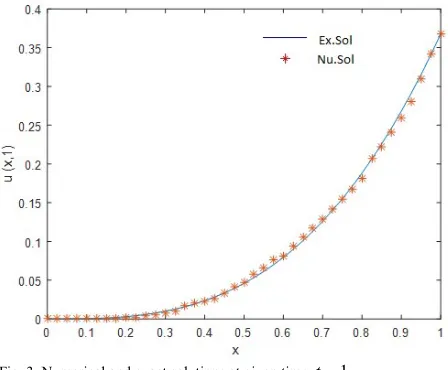
By the above difference scheme (17), the forward problem can be worked out. The numerical solutions and exact solution at time of t1are plotted in Fig.3. By Fig.3, we can see that the difference scheme given by (17) is of numerical convergence, and numerical solutions basically coincide with the exact solution.
Fig. 3. Numerical and exact solutions at given time t1.
(c) Source term inversion problem
We take the function q x t( , ) (1 x e x) t 3 e xt 3e xt 4
as the true source term, and apply the NACA to reconstruct its coefficient D
D D1, 2
1, 1
. We initially perform theinversion of two parameters without noise. The different inversion parameter intervals are as follows: 3 D11,
2
3 D 1
. Setting the number of niches to 4, the number of individuals is 100, the maximum iterations is 200, and the radius is still calculated according to (2). Similar to that in Section III, 50 runs are carried out to obtain an average result
IAENG International Journal of Applied Mathematics, 47:2, IJAM_47_2_11
[image:9.612.313.537.405.590.2]in the following simulations. Let us first investigate impacts of the algorithm parameters on the inversion algorithm, including the transition probability and the pheromone evaporation factor. Table XIV and Table XV show the inversed results of source term with different algorithm parameter. As shown in Table XIV, the optimal results go to be the best when the transition probability reaches 0.7, while the CPU time has no evident change. From the obtained inversed results in Table XV, it is indicated that when pheromone evaporation factor equals to 0.2, the inversion procedure finds the optimal results.
2 2
true inv true
[image:10.612.64.303.236.277.2]Err D D D denotes the relative error of the solution.
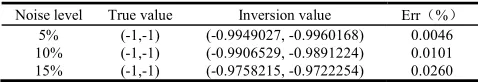
TABLE XVI The parameter inversion results with different levels of noise
Noise level True value Inversion value Err(%) 5% (-1,-1) (-0.9949027, -0.9960168) 0.0046 10% (-1,-1) (-0.9906529, -0.9891224) 0.0101 15% (-1,-1) (-0.9758215, -0.9722254) 0.0260
(d) Anti-noise property
For the purpose of examining the robustness and stability of NACA on the source term inversion, we will use measurement with different levels of noise: 5% noise, 10% noise, and 15% noise. These different levels of noise will be dealt with as follows:
*
, ,
1
obs j obs j
C
C
(18)
where is the noise level; * ,
obs j
C is the measured velocity
with noise;
is the random number according to standard normal distribution. In this process, the parameter values are the same as the foregoing example. Table XVI shows the inversion results. As we can see, the inversion results with different levels of noise are satisfactory.V. CONCLUSION
We numerically study the use of NACA for parameter estimation based on the space fractional order diffusion equation. This article shows that NACA is effective for multiparameter estimation. As shown in the examples, the proposed method has been successful at inverting parameters. The present work investigates the inversion of fractional order and source term involved in space fractional order diffusion equation. The numerical results show that the proposed method can provide accurate inversion solution for two-parameter inversion. To some extent, these results maybe can verify the effectiveness of the NACA for multiparameter identification of the space fractional order diffusion equation. Also shown in this paper is the result that the NACA inversion method possesses good performance to resist the noisy measurement data for the multiparameter estimation. With 5%, 10%, and 15% noises, the results obtained with the NACA are satisfactory.
[image:10.612.66.553.456.554.2]For the problem of parameter inversion of the space fractional order diffusion equation, some practical implementation issues still need to be resolved. Nevertheless, the better results obtained mean that there is good potential that the method can be employed to solve more complicated multiparameter inversion simultaneously. And this is an important direction for our future research.
TABLE XIV The inversion results with different transition probabilities Transition probability
1 , 1
true true
D D
1 , 1
inv inv
D D Err Time (s)
0.1 (-1,-1) (-0.9391825, -0.9424503) 0.0592 22.84521
0.2 (-1,-1) (-0.9436245, -0.9490321) 0.0537 23.29652
0.3 (-1,-1) (-0.9521436, -0.9561286) 0.0459 23.02153
0.4 (-1,-1) (-0.9259264, -0.9199013) 0.0772 22.90254
0.5 (-1,-1) (-1.0396982, -0.9601253) 0.0398 23.07454
0.6 (-1,-1) (-0.9785621, -0.9801325) 0.0206 23.04203
0.7 (-1,-1) (-0.9994781, -0.9991258) 0.0007 22.75255
0.8 (-1,-1) (-0.9792604, -0.9798153) 0.0204 22.80521
0.9 (-1,-1) (-0.9498702, -0.9391368) 0.0558 22.72989
TABLE XV The inversion results with different pheromone evaporation factors Pheromone evaporation
factors
1 , 1
true true
D D
1 , 1
inv inv
D D Err Time (s)
0.1 (-1,-1) (-0.987808, -0.9891224) 0.0115 23.184521
0.2 (-1,-1) (-0.9988197, -0.999208) 0.0010 23.22565
0.3 (-1,-1) (-0.9794781, -0.9802851) 0.0202 23.03252
0.4 (-1,-1) (-0.9612457, -0.9601812) 0.0393 23.09528
0.5 (-1,-1) (-0.9548711, -0.9485692) 0.0484 23.07454
0.6 (-1,-1) (-0.9711241, -0.9758023) 0.0267 23.04203
0.7 (-1,-1) (-0.9654212, -0.9582478) 0.0383 22.95645
0.8 (-1,-1) (-0.9800148, -0.9810256) 0.0195 22.88145
0.9 (-1,-1) (-0.9311087, -0.9286598) 0.0701 22.91809
IAENG International Journal of Applied Mathematics, 47:2, IJAM_47_2_11
[image:10.612.72.545.580.684.2]ACKNOWLEDGMENT
We thank the reviewers for their constructive comments in improving the quality of this paper.
REFERENCES
[1] J. Ma, “A new finite element analysis for inhomogeneous boundary-value problems of space fractional differential equations,” Journal of Scientific Computing, pp. 1–13, 2015.
[2] K. Sakamoto and M. Yamamoto, “Initial value/boundary value problems for fractional diffusion-wave equations and applications to some inverse problems,” Journal of Mathematical Analysis and Applications, vol. 382, no. 1, pp. 426–447, 2011.
[3] J. F. Huang, N. M. Nie, and Y. F. Tang, “A second order finite difference-spectral method for space fractional diffusion equations,” Science China Mathematics, vol. 57, no. 6, pp. 1303–1317, 2014. [4] M. Chen and W. Deng, “Fourth order accurate scheme for the space
fractional diffusion equations,” SIAM Journal on Numerical Analysis, vol. 52, no.31, pp. 1418–1438, 2014.
[5] M. Japundžić and D. Rajter-Ćirić, “Reaction-advection-diffusion equations with space fractional derivatives and variable coefficients on infinite domain,” Fractional Calculus & Applied Analysis, vol.18, no. 4, pp. 911–950, 2015.
[6] Q. Yang, F. Liu, and I. Turner, “Numerical methods for fractional partial differential equations with riesz space fractional derivatives ,” Applied Mathematical Modelling, vol. 34, no. 1, pp. 200–218, 2010. [7] A. Bouhassoun, “Multistage telescoping decomposition method for
solving fractional differential equations,” IAENG International Journal of Applied Mathematics, vol. 43, no. 1, pp. 10–16, 2013.
[8] M. Asgari, “Numerical solution for solving a system of fractional integro-differential equations,” IAENG International Journal of Applied Mathematics, vol. 45, no. 2, pp. 85–91, 2015.
[9] H. Song, M. Yi, J. Huang, and Y. Pan, “Bernstein polynomials method for a class of generalized variable order fractional differential equations,” IAENG International Journal of Applied Mathematics, vol. 46, no. 4, pp.437–444, 2016.
[10] J. Liu and M. Yamamoto, “A backward problem for the time-fractional diffusion equation,” Applicable Analysis, vol. 89, no. 11, pp. 1769–1788, 2010.
[11] G. H. Zheng and T. Wei, “Two regularization methods for solving a rieszcfeller space-fractional backward diffusion problem,” Inverse Problems, vol. 26, no. 11, pp. 115017–115038(22), 2010.
[12] Y. Zhang and X. Xu, “Inverse source problem for a fractional diffusion equation,” Inverse Problems, vol. 27, no. 3, pp. 35010–35021(12), 2011.
[13] F. A. Rodrigues, H. R. B. Orlande, and G. S. Dulikravich, “Simultaneous estimation of spatially dependent diffusion coefficient and source term in a nonlinear 1D diffusion problem,” Mathematics and Computers in Simulation, vol. 66, no. 4, pp. 409–424, 2004. [14] Cheng, Jin, Nakagawa, Junichi, Yamamoto, Masahiro, Yamazaki, and
Tomohiro, “Uniqueness in an inverse problem for a one-dimensional fractional diffusion equation,” Inverse Problems, vol. 25, no. 11, pp. 115017–115032(16), 2009.
[15] A. N. Bondarenko and D. S. Ivaschenko, “Numerical methods for solving inverse problems for time fractional diffusion equation with variable coefficient,” Journal of Inverse and Ill-posed Problems, vol. 17, no. 5, pp. 419–440, 2009.
[16] P. Rocca, M. Benedetti, M. Donelli, D. Franceschini, and A. Massa, “Evolutionary optimization as applied to inverse scattering problems,” Inverse Problems, vol. 25, no. 12, pp. 1541–1548, 2009.
[17] X. Xie and X. Li, “Genetic algorithm-based tension identification of hanger by solving inverse eigenvalue problem,” Inverse Problems in Science and Engineering, vol. 22, no. 6, pp. 966–987, 2014.
[18] A. Laudani, G. Pulcini, F. R. Fulginei, and A. Salvini, “Electric circuits performing the swarm optimization,” Inverse Problems in Science and Engineering, vol. 22, no. 7, pp. 1109–1127, 2014.
[19] A. Colorni, M. Dorigo, and V. Maniezzo, “Distributed optimization by ant colonies,” in Ecal91 - European Conference on Artificial Life, 1991, pp. 134–142.
[20] G. Bilchev and I. C. Parmee, “The ant colony metaphor for searching continuous design spaces,” Lecture Notes in Computer Science, vol.993, pp. 25–39, 1995.
[21] Y. J. Li and T. J. Wu, “An adaptive ant colony system algorithm for continuous-space optimization problems,” Journal of Zhejiang University-SCIENCE A, vol. 4, no. 1, pp. 40–46, 2003.
[22] C. Ling, S. Jie, Q. Ling, and C. Hongjian, “A method for solving optimization problems in continuous space using ant colony algorithm,” in Ant Algorithms, Third International Workshop, ANTS 2002, Brussels, Belgium, September 12-14, 2002, Proceedings, 2002, pp. 2317–2323.
[23] J. Dro and P. Siarry, “Continuous interacting ant colony algorithm based on dense heterarchy,” Future Generation Computer Systems, vol. 20, no. 5, pp. 841–856, 2004.
[24] J. Dro and P. Siarry,, “An ant colony algorithm aimed at dynamic continuous optimization,” Applied Mathematics and Computation, vol. 181, no. 1, pp. 457–467, 2006.
[25] C. Ye, “Ant colony system for continuous function optimization,” Journal of Sichuan University, vol. 36, no. 6, pp. 117–120, 2004. [26] Y. Zhang and S. Huang, “On ant colony algorithm for solving
multiobjective optimization problems,” Control and Decision, vol. 20, no. 2, pp. 170–173, 2005. (in Chinese)
[27] S. W. Mahfoud, “Crowding and preselection revisited,” Parallel Problem Solving from Nature, Amsterdam, North-Holland, 1992, pp. 27–36.
[28] D. E. Goldberg and J. Richardson, “Genetic algorithms with sharing for multimodal function optimization,” in International Conference on Genetic Algorithms on Genetic Algorithms and Their Application, 1987, pp. 41–49.
[29] A. Trowski, “A clearing procedure as a niching method for genetic algorithms,” in IEEE International Conference on Evolutionary Computation, 1996, pp. 798–803.
[30] F. Streichert, G. Stein, H. Ulmer, and A. Zell, “A clustering based niching ea for multimodal search spaces,” in Artificial Evolution, International Conference, Evolution Artificielle, 2003, pp. 293–304. [31] B. L. Miller and M. J. Shaw, “Genetic algorithms with dynamic niche
sharing for multimodal function optimization,” in IEEE International Conference on Evolutionary Computation, 1996, pp. 786–791. [32] B. Sareni and L. Krähenbühl, “Fitness sharing and niching methods
revisited,” IEEE Transactions on Evolutionary Computation, vol. 2, no. 3, pp. 97–106, 1998.
[33] A. Della Cioppa, C. De Stefano, and A. Marcelli, “On the role of population size and niche radius in fitness sharing,” IEEE Transactions on Evolutionary Computation, vol. 8, no. 6, pp. 580–592, 2005. [34] D. J. Cavicchio, “Adaptive search using simulated evolution,” Umr,
1970.
[35] D. Angus, “Niching for population-based ant colony optimization,” in IEEE International Conference on E-Science and Grid Computing, 2006. E-Science, 2006, pp. 115–115.
[36] D. Angus, “Crowding population-based ant colony optimisation for the multi-objective travelling salesman problem,” in Computational Intelligence in Multicriteria Decision Making, IEEE Symposium on, 2007, pp. 333–340.
[37] J. Andre, P. Siarry, and T. Dognon, “An improvement of the standard genetic algorithm fighting premature convergence in continuous optimization,” Advances in Engineering Software, vol. 32, no. 1, pp. 49–60, 2001
[38] R. S. Anderssen, “Global optimization,” Optimization, pp. 26–48, 1972.
IAENG International Journal of Applied Mathematics, 47:2, IJAM_47_2_11
[39] A. H. G. R. Kan and G. T. Timmer, “Stochastic global optimization methods part ii: Multi level methods,” Mathematical Programming, vol. 39, no. 1, pp. 57–78, 1987.
[40] F. Aluffi-Pentini, V. Parisi, and F. Zirilli, “Global optimization and stochastic differential equations,” Journal of Optimization Theory and Applications, vol. 47, no. 1, pp. 1–16, 1985.
[41] A. Dekkers and E. Aarts, “Global optimization and simulated annealing,” Mathematical Programming, vol. 50, no. 1, pp. 367–393, 1991.
[42] D. Cvijović and J. Klinowski, “Taboo search: An approach to the multiple minima problem,” Science, vol. 267, no. 267, pp. 664–666, 1995.
DATE OF MODIFICATION:10/6/2017
BRIEF DESCRIPTION OF THE CHANGES: ADD SENTENCE
“RADIUS IS STILL CALCULATED ACCORDING TO (2).SIMILAR TO THAT IN SECTION III,50 RUNS ARE CARRIED OUT TO OBTAIN AN AVERAGE RESULT IN THE FOLLOWING SIMULATIONS.LET US FIRST INVESTIGATE IMPACTS OF THE ALGORITHM PARAMETERS ON THE INVERSION ALGORITHM, INCLUDING THE” ON THE LEFT TOP OF PAGE 10,WHICH MISSED IN THE ONLINE VERSION.