Neural Particle Smoothing for Sampling from Conditional Sequence Models

Proceedings of NAACL-HLT 2018, pages 929–941

Neural Particle Smoothing

for Sampling from Conditional Sequence Models

Center for Language and Speech Processing Johns Hopkins University, Baltimore MD, 21218

{kitsing,jason}@cs.jhu.edu

Abstract

We introduce neural particle smoothing, a sequential Monte Carlo method for sampling annotations of an input string from a given probability model. In contrast to conventional particle filtering algorithms, we train a proposal distribution that looks ahead to the end of the input string by means of a right-to-left LSTM. We demonstrate that this innovation can improve the quality of the sample. To motivate our formal choices, we explain how our neural model and neural sampler can be viewed as low-dimensional but nonlinear approximations to working with HMMs over very large state spaces.

1 Introduction

Many structured prediction problems in NLP can be reduced to labeling a length-T input string x

with a length-T sequenceyof tags. In some cases,

these tags are annotations such as syntactic parts of speech. In other cases, they represent actions that incrementally build an output structure: IOB tags build a chunking of the input (Ramshaw and Marcus,

1999), shift-reduce actions build a tree (Yamada and Matsumoto,2003), and finite-state transducer arcs build an output string (Pereira and Riley,1997).

One may wish to score the possible taggings us-ing a recurrent neural network, which can learn to be sensitive to complex patterns in the training data. A globally normalized conditional probability model is particularly valuable because it quantifies uncer-tainty and does not suffer from label bias (Lafferty et al.,2001); also, such models often arise as the predictive conditional distributionp(y _| x) corre-sponding to some well-designed generative model

p(x,y)for the domain. In the neural case, however, inference in such models becomes intractable. It is hard to know what the model actually predicts and hard to compute gradients to improve its predictions.

In such intractable settings, one generally falls back on approximate inference or sampling. In the NLP community, beam search and importance

sam-pling are common. Unfortunately, beam search con-siders only the approximate-top-k taggings from

an exponential set (Wiseman and Rush,2016), and importance sampling requires the construction of a good proposal distribution (Dyer et al.,2016).

In this paper we exploit the sequential structure of the tagging problem to dosequentialimportance sampling, which resembles beam search in that it constructs its proposed samples incrementally—one tag at a time, taking the actual model into account at every step. This method is known as particle filtering (Doucet and Johansen,2009). We extend it here to take advantage of the fact that the sampler has access to the entire input string as it constructs its tagging, which allows it to look ahead or—as we will show— to use a neural network to approximate the effect of lookahead. Our resulting method is calledneural particle smoothing.

1.1 What this paper provides

Forx= x1· · ·xT, letx:tandxt:respectively

de-note the prefixx1· · ·xtand the suffixxt+1· · ·xT.

We develop neural particle smoothing—a se-quential importance sampling method which, given a string x, draws a sample of taggings y from pθ(y| x). Our method works for any conditional

probability model of the quite general form1

pθ(y|x)

def

∝expGT (1)

whereGis anincremental stateful global scoring

modelthat recursively defines scoresGtof prefixes

of(x,y)at all times0≤t≤T:

Gt=def Gt−1+gθ(st−1, xt, yt) (withG0 def= 0) (2)

st=def fθ(st−1, xt, yt) (withs0given) (3)

These quantities implicitly depend onx,yandθ.

Herestis the model’sstateafter observing the pair

of length-tprefixes(x:t,y:t).Gtis thescore-so-far

1_{A model may require for convenience that each input end} with a special end-of-sequence symbol: that is,xT=EOS.

of this prefix pair, whileGT −Gtis the

score-to-go. The statestsummarizes the prefix pair in the

sense that the score-to-go depends only onstand the

length-(T₋t)suffixes(xt:,yt:). Thelocal scoring

function gθ and state update function fθ may be

any functions parameterized byθ—perhaps neural

networks. We assumeθis fixed and given.

This model family is expressive enough to capture any desiredp(y _|x). Why? Take any distribution p(x,y) with this desired conditionalization (e.g., the true joint distribution) and factor it as

logp(x,y) =PT_t=1logp(xt, yt|x:t−1,y:t−1)

=PT_t=1logp(xt, yt|st−1)

| {z }

use asgθ(st−1,xt,yt)

=GT (4)

by makingst include as much information about

(x:t,y:t)as needed for (4) to hold (possibly st =

(x:t,y:t)).2Then by defininggθas shown in (4), we

getp(x,y) = expGT and thus (1) holds for each

x.

1.2 Relationship to particle filtering

Our method is spelled out in§4(one may look now). It is a variant of the popularparticle filteringmethod that tracks the state of a physical system in discrete time (Ristic et al.,2004). Our particularproposal distributionforytcan be found in equations (5), (6),

(25) and (26). It considers not only past observations

x:tas reflected inst−1, but also future observations

xt:, as summarized by the state¯stof a right-to-left

recurrent neural network_f¯_{that we will train:}

ˆ

Htdef=hφ(¯st+1, xt+1) + ˆHt+1 (5)

¯

stdef= ¯fφ(¯st+1, xt+1) (withsT given) (6)

Conditioning the distribution ofyton future

obser-vationsxt:means that we are doing “smoothing”

rather than “filtering” (in signal processing terminol-ogy). Doing so can reduce the bias and variance of our sampler. It is possible so long asxis provided in

its entirety before the sampler runs—which is often the case in NLP.

1.3 Applications

Why sample from pθ at all? Many NLP systems

instead simply search for theViterbi sequenceythat

maximizesGT and thus maximizes pθ(y | x). If

the space of statessis small, this can be done effi-ciently by dynamic programming (Viterbi,1967); if

2_{Furthermore,stcould even depend on all ofx(ifs} 0does), allowing direct expression of models such as stacked BiRNNs.

not, thenA∗ may be an option (see§2). More com-mon is to use an approximate method: beam search, or perhaps a sequential prediction policy trained with reinforcement learning. Past work has already shown how to improve these approximate search algorithms by conditioning on the future (Bahdanau et al.,2017;Wiseman and Rush,2016).

Sampling is essentially a generalization of maximization: sampling from exp GT

temperature

approaches maximization astemperature_→0. It is a fundamental building block for other algorithms, as it can be used to take expectations over the whole space of possibleyvalues. For unfamiliar readers, AppendixEreviews how sampling is crucially used in minimum-risk decoding, supervised training, unsupervised training, imputation of missing data, pipeline decoding, and inference in graphical models.

2 Exact Sequential Sampling

To develop our method, it is useful to first consider exact samplers. Exact sampling is tractable for only some of the models allowed by§1.1. However, the form and notation of the exact algorithms in§2will guide our development of approximations in§3.

An exact sequential sampler draws yt from

pθ(yt|x,y:t−1)for eacht= 1, . . . , T in sequence.

Thenyis exactly distributed aspθ(y|x).

For each givenx,y_:t−1, observe that

pθ(yt|x,y:t−1) (7)

∝pθ(y:t|x) = P

yt:pθ(y|x) (8)

∝Pyt:expGT (9)

= exp (Gt+ logP_yt:exp (GT −Gt)

| {z }

call thisHt

)(10)

= exp (Gt−1+gθ(st−1, xt, yt) +Ht) (11)

∝exp (gθ(st−1, xt, yt) +Ht) (12)

Thus, we can easily construct the needed distribu-tion (7) by normalizing (12) over all possible values ofyt. The challenging part of (12) is to computeHt:

as defined in (10),Htinvolves a sum over

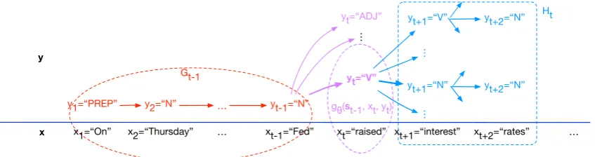
exponen-tially many futuresy_t:. (See Figure1.)

We chose the symbols GandH in homage to

theA∗search algorithm (Hart et al.,1968). In that

algorithm (which could be used to find the Viterbi sequence),g denotes the score-so-far of a partial

solution y_:t, and h denotes the optimal

score-to-go. Thus,g +h would be the score of the best

x1=“On” x2=“Thursday” … _{xt-1=“Fed” xt=“raised” xt+1=“interest” xt+2=“rates”} …

y1=“PREP” y2=“N” … yt-1=“N”

yt=“ADJ”

…

yt=“V”

yt+1=“V”

…

yt+1=“N”

…

yt+2=“N”

yt+2=“N” Ht

x y

g_θ(s_{t-1, xt, yt)} Gt-1

Figure 1: Sampling a single particle from a tagging model.y1, . . . , yt−1 (orange) have already been chosen, with a total model score ofGt−1, and now the sampler is constructing a proposal distributionq(purple) from which the next tagytwill be

sampled. Eachytis evaluated according to its contribution toGt(namelygθ) and its future scoreHt(blue). The figure illustrates

quantities used throughout the paper, beginning with exact sampling in equations (7)–(12). Our main idea (§3) is toapproximate

theHtcomputation (a log-sum-exp over exponentially many sequences) when exact computation by dynamic programming is

not an option. The form of our approximation uses a right-to-left recurrent neural network but isinspiredby the exact dynamic programming algorithm.

Htis the log of the total exponentiated scores of

allsequences with prefixy_:t.GtandHtmight be

called thelogprob-so-farandlogprob-to-goofy_:t.

Just asA∗approximateshwith a “heuristic”ˆh,

the next section will approximateHtusing a neural

estimate_Hˆ_{t(equations (5)–(6)). However, the} spe-cific form of our approximation is inspired by cases where Htcan be computed exactly. We consider

those in the remainder of this section.

2.1 Exact sampling from HMMs

A hidden Markov model (HMM) specifies a nor-malizedjointdistributionpθ(x,y) = expGT over

state sequenceyand observation sequencex,3Thus

the posteriorpθ(y |x)is proportional toexpGT,

as required by equation (1).

The HMM specifically defines GT by

equa-tions (2)–(3) withst = ytandgθ(st−1, xt, yt) =

logpθ(yt|yt−1) + logpθ(xt|yt).4

In this setting,Ht can be computed exactly by

thebackward algorithm(Rabiner,1989). (Details are given in AppendixAfor completeness.) 2.2 Exact sampling from OOHMMs

For sequence tagging, a weakness of (first-order) HMMs is that the model statest=ytmay contain

little information: only the most recent tag yt is

remembered, so the number of possible model states

stis limited by the vocabulary of output tags.

We may generalize so that the data generating process is in a latent stateut ∈ {1, . . . , k}at each

timet, and the observedyt—along withxt—is

gen-erated fromut. Nowkmay be arbitrarily large. The

3_{The HMM actually specifies a distribution over a pair of} in-finite sequences, but here we consider the marginal distribution over just the length-Tprefixes.

4_{It takess}

0 =BOS, a beginning-of-sequence symbol, so pθ(y1 |BOS)specifies the initial state distribution.

model has the form

pθ(x,y) = expGT (13)

=X

u

T Y

t=1

pθ(ut|ut−1)·pθ(xt, yt|ut)

This is essentially a pair HMM (Knudsen and Miyamoto,2003) without insertions or deletions, also known as an “-free” or “same-length”

proba-bilistic finite-state transducer. We refer to it here as anoutput-output HMM(OOHMM).5

Is this still an example of the general model ar-chitecture from §1.1? Yes. Since utis latent and

evolves stochastically, it cannot be used as the state

stin equations (2)–(3) or (4). However, wecan

de-finestto be the model’sbelief stateafter observing

(x:t,y:t). The belief state is the posterior probability

distribution over the underlying stateutof the

sys-tem. That is,stdeterministically keeps track of all

possible states that the OOHMM might be in—just as the state of a determinized FSA keeps track of all possible states that the original nondeterministic FSA might be in.

We may compute the belief state in terms of a vector offorward probabilitiesthat starts atα0,

(α0)u =def (

1 ifu=BOS(see footnote4) 0 ifu=any other state (14) and is updated deterministically for each0< t≤T

by theforward algorithm(Rabiner,1989):

(αt)u =def k X

u0₌₁

(αt−1)u0·pθ(u|u0)·pθ(xt, yt|u)

(15) 5_{This is by analogy with theinput-output HMM(IOHMM)} ofBengio and Frasconi(1996), which definesp(y|x)directly and conditions the transition toutonxt. The OOHMM instead

definesp(y_|x)by conditionalizing (13)—which avoids the

(αt)ucan be interpreted as the logprob-so-farif the

system is in stateuafter observing(x:t,y:t). We

may express the update rule (15) byα>_t =α>_t−1P

where the matrix P depends on (xt, yt), namely

Pu0_u def=p_θ(u|u0)·p_θ(x_t, y_t|u).

The belief state st =def JαtK ∈ Rk simply

nor-malizesαtinto a probability vector, whereJuKdef=

u/(u>1)denotes thenormalization operator. The state update (15) now takes the form (3) as desired, withfθa normalized vector-matrix product:

s>_t =fθ(st−1, xt, yt)=def Js>t−1PK (16)

As in the HMM case, we defineGtas the log of

the generative prefix probability,

Gt= logdef pθ(x:t,y:t) = log P

u(αt)u (17)

which has the form (2) as desired if we put

gθ(st−1, xt, yt)=def Gt−Gt−1 (18)

= logα

>

t−1P1

α>

t−11

= log (s>_t−1P1)

Again, exact sampling is possible. It suffices to compute (9). For the OOHMM, this is given by

P

yt:expGT =α

>

tβt (19)

whereβ_T =def 1and thebackward algorithm

(β_t)v =def pθ(xt:|ut=u) (20)

= X

ut:,yt:

pθ(ut:,xt:,yt:|ut=u)

=X

u0

pθ(u0 |u)·p(xt+1|u0)

| {z }

call thisPuu0

·(β_t+1)u0

for0_≤t < T uses dynamic programming to find

the total probability of all ways to generate the fu-ture observationsxt:. Note thatαtis defined for

a specific prefixy_:t (though it sums over allu:t),

whereasβ_tsums overall suffixesy_t:(and over all

ut:), to achieve the asymmetric summation in (19).

Define¯st def=JβtK∈Rk to be a normalized

ver-sion ofβ_t. Theβ_trecurrence (20) can clearly be ex-pressed in the form¯st=JP¯st+1K, much like (16).

2.3 The logprob-to-go for OOHMMs

Let us now work out the definition of Ht for

OOHMMs (cf. equation (35) in Appendix A for HMMs). We will write it in terms of_Hˆ_tfrom§1.2. Let us define_Hˆ_{tsymmetrically toGt(see (17)):}

ˆ

Htdef= log X

u

(β_t)u (= log1>βt) (21)

which has the form (5) as desired if we put

hφ(¯st+1, xt+1)= ˆdefHt−Hˆt+1 = log (1>P¯st+1)

(22)

From equations (10), (17), (19) and (21), we see

Ht= log X

yt:

expGT

−Gt

= log α>t βt (α>_t1)(1>_β

t)

+ log (1>β_t)

= logs>_t¯st | {z }

call thisCt

+ ˆHt (23)

where Ct ∈ Rcan be regarded as evaluating the

compatibilityof the state distributionsstand¯st.

In short, the generic strategy (12) for exact sam-pling says that for an OOHMM,ytis distributed as

pθ(yt|x,y:t−1)∝exp (gθ(st−1, xt, yt) +Ht)

∝exp (gθ(st−1, xt, yt)

| {z }

depends onx:t,y:t

+ _|{z}Ct

onx,y:t

+ ˆ_|{z}Ht

onxt: )

∝exp (gθ(st−1, xt, yt) +Ct) (24)

This is equivalent to choosingytin proportion to

(19)—but we now turn to settings where it is infea-sible to compute (19) exactly. There we will use the formulation (24) but approximateCt. For

com-pleteness, we will also consider how to approximate ˆ

Ht, which dropped out of the above distribution

(because it was the same for all choices ofyt) but

may be useful for other algorithms (see§4).

3 Neural Modeling as Approximation

3.1 Models with large state spaces

The expressivity of an OOHMM is limited by the number of statesk. The stateut ∈ {1, . . . , k}is a

bottleneck between the past(x:t,y:t)and the future

(xt:,yt:), in that past and future areconditionally

independentgivenut. Thus, the mutual information

between past and future is at mostlog₂kbits.

In many NLP domains, however, the past seems to carry substantial information about the future. The first half of a sentence greatly reduces the un-certainly about the second half, by providing infor-mation about topics, referents, syntax, semantics, and discourse. This suggests that an accurate HMM language modelp(x)would requirevery largek—

the information for predictingy_t:might be available inxt:. Still, it is important to let(x:t,y:t)contribute

enough additional information abouty_t:: even for

short strings, makingktoo small (giving≤log₂k

bits) may harm prediction (Dreyer et al.,2008). Of course, (4) says that an OOHMM can express any joint distribution for which the mutual informa-tion is finite,6_{by takingklarge enough forv}

t−1to

capture the relevant info from(x:t−1,y:t−1).

So why not just takekto be large—say,k= 230 to allow 30 bits of information? Unfortunately, eval-uatingGT then becomes very expensive—both

com-putationally and statistically. As we have seen, if we define stto be the belief stateJαtK∈ Rk,

up-dating it at each observation(xt, yt)(equation (3))

requires multiplication by ak×kmatrixP. This

takes timeO(k2), and requires enough data to learn O(k2_{)transition probabilities.}

3.2 Neural approximation of the model As a solution, we might hope that for the inputs

xobserved in practice, the very high-dimensional

belief statesJαtK∈Rk might tend to lie near ad

-dimensional manifold wheredk. Then we could

takestto be a vector inRdthat compactly encodes

the approximate coordinates ofJαtKrelative to the

manifold:st=ν(JαtK), whereν is the encoder.

In this new, nonlinearly warped coordinate sys-tem, the functions ofst−1in (2)–(3) are no longer

the simple, essentially linear functions given by (16) and (18). They become nonlinear functions operat-ing on the manifold coordinates. (fθin (16) should

now ensure thats>_t ≈ν(_J(ν−1(st−1))>PK), andgθ

in (18) should now estimatelog (ν−1(st−1))>P1.)

In a sense, this is the reverse of the “kernel trick” (Boser et al.,1992) that converts a low-dimensional nonlinear function to a high-dimensional linear one.

Our hope is thatsthas enough dimensionsdk

to capture the useful information from the trueJαtK,

andthatθhas enough dimensionsk2to capture

most of the dynamics of equations (16) and (18). We thus proceed to fit the neural networksfθ, gθ

directly to the data,without ever knowingthe truek

or the structure of the original operatorsP ∈Rk×k_.

We regard this as the implicit justification for various published probabilistic sequence models

pθ(y|x)that incorporate neural networks. These

models usually have the form of§1.1. Most simply, (fθ, gθ)can be instantiated as one time step in an

RNN (Aharoni and Goldberg,2017), but it is com-6_{This is not true for the language of balanced parentheses.}

mon to use enriched versions such as deep LSTMs. It is also common to have the statestcontain not

only a vector of manifold coordinates inRd_{but also}

some unboundedly large representation of(x,y_:t) (cf. equation (4)), so thefθneural network can refer

to this material with an attentional (Bahdanau et al.,

2015) or stack mechanism (Dyer et al.,2015). A few such papers have usedgloballynormalized conditional models that can be viewed as approx-imating some OOHMM, e.g., the parsers ofDyer et al.(2016) andAndor et al. (2016). That is the case (§1.1) that particle smoothing aims to support. Most papers are locally normalized conditional models (e.g.,Kann and Schütze,2016;Aharoni and Goldberg,2017); these simplify supervised training and can be viewed as approximating IOHMMs (footnote5). For locally normalized models,Ht= 0

by construction, in which case particle filtering (which estimatesHt= 0) is just as good as particle

smoothing. Particle filtering is still useful for these models, but lookahead’s inability to help them is an expressive limitation (known aslabel bias) of locally normalized models. We hope the existence of particle smoothing (which learns an estimate

Ht) will make it easier to adopt, train, and decode

globally normalized models, as discussed in§1.3. 3.3 Neural approximation of logprob-to-go We can adopt the same neuralization trick to approx-imate the OOHMM’s logprob-to-goHt=Ct+ ˆHt.

We take¯st∈Rdon the same theory that it is a

low-dimensional reparameterization ofJβtK, and define

( ¯fφ, hφ)in equations (5)–(6) to be neural networks.

Finally, we must replace the definition ofCtin (23)

with another neural networkcφthat works on the

low-dimensional approximations:7

Ct=def cφ(st,¯st) (except thatCT = 0)def (25)

The resulting approximation to (24) (which does not actually requirehφ) will be denotedqθ,φ:

qθ,φ(yt|x,y:t−1)

def

∝exp (gθ(st−1, xt, yt) +Ct)

(26) The neural networks in the present section are all parameterized byφ, and are intended to produce an

estimate of the logprob-to-goHt—a function ofxt:,

which sums over all possibley_t:.

By contrast, the OOHMM-inspired neural networks suggested in§3.2were used to specify an

7_C

actual model of the logprob-so-farGt—a function

ofx:tandy:t—using separate parametersθ.

Arguably φ has a harder modeling job than θ

because it must implicitly sum over possible futures

y_t:. We now consider how to get corrected samples

fromqθ,φ even ifφgives poor estimates ofHt, and

then how to trainφto improve those estimates.

4 Particle smoothing

In this paper, we assume nothing about the given model GT except that it is given in the form of

equations (1)–(3) (including the parameter vectorθ).

Suppose we run the exact sampling strategy but approximatepθin (7) with aproposal distribution

qθ,φof the form in (25)–(26). Suppressing the

sub-scripts on p andq for brevity, this means we are

effectively drawingynot fromp(y_|x)but from

q(y_|x) =

T Y

t=1

q(yt|x,y:t−1) (27)

IfCt≈Ht+const within eachytdraw, thenq ≈p.

Normalized importance sampling corrects (mostly) for the approximation by drawingmany se-quencesy(1)_{, . . .y}(M)_{IID from (27) and assigning}

y(m) _{a relativeweightofw}(m) ₌def p(y(m)_|x)

q(y(m)_|x). This ensemble of weighted particlesyields a distribution

ˆ

p(y)=def

PM

m=1_PMw(m)I(y=y(m))

m=1w(m) ≈

p(y|x) (28)

that can be used as discussed in §1.3. To com-pute w(m) in practice, we replace the numerator p(y(m) _{|x)by the unnormalized versionexpG}

T,

which gives the samepˆ. Recall that eachGT is a

sumPT

t=1gθ(· · ·).

Sequential importance samplingis an equivalent implementation that makesttheouterloop andm

theinnerloop. It computes aprefix ensemble

Yt

def

={(y(1)_:t , w_t(1)), . . . ,(y(_:tM), w_t(M))} (29)

for each 0 _≤ t _≤ T in sequence. Initially, (y(_:0m), w₀(m)) = (,expC0) for all m. Then for

0< t_≤T, we extend these particles in parallel:

y_:(_tm)=y(_:tm₋)₁y(_tm) (concatenation) (30)

w_t(m)=w_t(₋m₁) exp (gθ(st−1,xt,yt) +Ct−Ct−1)

q(yt|x,y:t−1) (31)

where eachy_t(m)is drawn from (26). EachYtyields

a distributionpˆtover prefixesy:t, which estimates

the distributionpt(y:t)

def

∝exp (Gt+Ct). We return

ˆ

p = ˆdef pT ≈ pT = p. This gives the same pˆas in

(28): the final y(_Tm) are the same, with the same

final weightsw(_Tm)= expGT

q(y(m)_|x), whereGT was now summed up asC0+PTt=1gθ(· · ·) +Ct−Ct−1.

That is our basicparticle smoothingstrategy. If we use the naive approximationCt= 0everywhere,

it reduces toparticle filtering. In either case, various well-studied improvements become available, such as various resampling schemes (Douc and Cappé,

2005) and the particle cascade (Paige et al.,2014).8

An easy improvement ismultinomial resampling. After computing eachpˆt, this replacesYtwith a set

ofM new draws frompˆt(≈ pt), each of weight

1—which tends to drop low-weight particles and duplicate high-weight ones.9 _{For this to usefully}

focus the ensemble on good prefixesy_:t,ptshould

be a good approximation to the true marginal

p(y_:t|x)_∝exp (Gt+Ht)from (10). That is why

we arranged forpt(y:t)∝exp (Gt+Ct). Without

Ct, we would have onlypt(y:t)∝expGt—which

is fine for the traditional particle filtering setting, but in our setting it ignores future information inxt:

(which we have assumed is available) and also fa-vors sequencesythat happen to accumulate most of

their global scoreGT early rather than late (which

is possible when the globally normalized model (1)–(2) isnotfactored in the generative form (4)).

5 Training the Sampler Heuristic

We now consider training the parametersφof our

sampler. These parameters determine the updates_f¯_φ in (6) and the compatibility functioncφin (25). As

a result, they determine the proposal distributionq

used in equations (27) and (31), and thus determine the stochastic choice ofpˆthat is returned by the sampler on a given inputx.

In this paper, we simply try to tune φto yield

good proposals. Specifically, we try to ensure that

qφ(y|x)in equation (27) is close top(y|x)from

equation (1). While this may not be necessary for the sampler to perform well downstream,10_{it does}

8_{The particle cascade would benefit from an estimate ofHˆ}

t,

as it (like A∗_{search) compares particles of different lengths.}

9_{While resampling mitigates the degeneracy problem, it} could also reduce the diversity of particles. In our experiments in this paper, we only do multinomial resampling when the ef-fective sample size ofpˆtis lower thanM₂.Doucet and Johansen

“na-guarantee it (assuming that the modelpis correct). Specifically, we seek to minimize

(1₋λ)KL(p_||qφ) +λKL(qφ||p) (withλ∈[0,1])

(32) averaged over examples xdrawn from a training

set.11_{(The training set need not provide truey’s.)}

Theinclusive KL divergenceKL(p||qφ)is an

ex-pectation underp. We estimate it by replacingpwith

a samplepˆ, which in practice we can obtain with our sampler under the currentφ. (The danger, then, is

thatpˆwill be biased whenφis not yet well-trained;

this can be mitigated by increasing the sample size

M when drawingpˆfor training purposes.)

Intuitively, this term tries to encourageqφin

fu-ture to re-propose thoseyvalues that turned out to

be “good” and survived intopˆwith high weights. The exclusive KL divergence KL(qφ||p) is an

expectation underqφ. Since we can sample from

qφ exactly, we can get an unbiased estimate of

∇φKL(qφ||p)with the likelihood ratio trick (Glynn,

1990).12 _{(The danger is that such “REINFORCE”}

methods tend to suffer from very high variance.) This term is a popular objective for variational approximation. Here, it tries to discourageqφfrom

re-proposing “bad”yvalues that turned out to have

lowexpGT relative to their proposal probability.

Our experiments balance “recall” (inclusive) and “precision” (exclusive) by takingλ= 1₂ (which

Ap-pendixFcompares toλ∈ {0,1}). Alas, because of our approximation to the inclusive term, neither term’s gradient will “find” and directly encourage goodyvalues that have never been proposed.

Ap-pendixBgives further discussion and formulas.

6 Models for the Experiments

To evaluate our methods, we needed pre-trained modelspθ. We experimented on several models. In

each case, we trained agenerativemodelpθ(x,y),

so that we could try sampling from its posterior dis-tributionpθ(y|x). This is a very common setting

where particle smoothing should be able to help. Details for replication are given in AppendixC. tural” goal of sampling. This objective can tolerate inaccurate local proposal distributions in cases where the algorithm could recover from them through resampling. Looking even farther downstream, we might merely wantpˆ—which is typically used to compute expectations—to provide accurate guidance to some decision or training process (see AppendixE). This might not require fully matching the model, and might even make it desir-able to deviate from an inaccurate model.

11_{Training a single approximationq}

φfor allxis known as amortized inference.

12_{The normalizing constant ofpfrom (1) can be ignored} because the gradient of a constant is 0.

6.1 Tagging models

We can regard a tagged sentence(x,y)as a string over the “pair alphabet”X × Y. We train an RNN language model over this “pair alphabet”—this is a neuralized OOHMM as suggested in§3.2:

logpθ(x,y) = T X

t=1

logpθ(xt, yt|st−1) (33)

This model is locally normalized, so that logpθ(x,y)(as well as its gradient) is

straightfor-ward to compute for a given training pair (x,y).

Joint sampling from it would also be easy (§3.2). However,p(y|x)is globally renormalized (by an unknown partition function that depends onx,

namelyexpH0). Conditional sampling ofyis

there-fore potentially hard. Choosing yt optimally

re-quires knowledge ofHt, which depends on the

fu-turext:.

As we noted in§1, many NLP tasks can be seen as tagging problems. In this paper we experiment with two such tasks:English stressed syllable tagging, where the stress of a syllable often depends on the number of remaining syllables,13 _{providing good}

reason to use thelookaheadprovided by particle smoothing; andChinese NER, which is a familiar textbook application and reminds the reader that our formal setup (tagging) provides enough machinery to treat other tasks (chunking).

English stressed syllable tagging This task tags a sequence of phonemes x, which form a word, with their stress markingsy. Our training examples

are the stressed words in the CMU pronunciation dictionary (Weide,1998). We test the sampler on held-out unstressed words.

Chinese social media NER This task does named entity recognition in Chinese, by tagging the characters of a Chinese sentence in a way that marks the named entities. We use the dataset from

Peng and Dredze(2015), whose tagging scheme is a variant of the BIO scheme mentioned in§1. We test the sampler on held-out sentences.

6.2 String source separation

This is an artificial task that provides a discrete ana-logue of speech source separation (Zibulevsky and Pearlmutter,2001). The generative model is thatJ

IID from an RNN language model, and are then combined into a single stringxaccording to a

ran-dominterleavingstringy.14The posteriorp(y_|x) predicts the interleaving string, which suffices to re-construct the original strings. The interleaving string is selected from the uniform distribution over all pos-sible interleavings (given theJstrings’ lengths). For

example, withJ = 2, a possible generative story is

that we first sample two stringsFooandBarfrom an RNN language model. We then draw an interleav-ing strinterleav-ing112122from the aforementioned uniform distribution, and interleave theJ strings

determinis-tically to getFoBoar.

p(x,y)is proportional to the product of the prob-abilities of the J strings. The only parameters of pθ, then, are the parameters of the RNN language

model, which we train on clean (non-interleaved) samples from a corpus. We test the sampler on ran-dom interleavings of held-out samples.

The states(which is provided as an input tocθ

in (25)) is the concatenation of theJ states of the

language model as it independently generates theJ

strings, andgθ(st−1, xt, yt)is the log-probability of

generatingxtas the next character of theytthstring,

given that string’s language model state withinst−1.

As a special case,xT =EOS(see footnote1), and

gθ(sT−1,EOS,EOS)is the total log-probability of

termination in allJ language model states. String source separation has good reason for lookahead: appending character “o” to a recon-structed string “ gh” is only advisable if “s” and “t” are coming up soon to make “ghost.” It also

il-lustrates a powerful application setting—posterior inference under a generative model. This task conve-niently allowed us to construct the generative model from a pre-trained language model. Our constructed generative model illustrates that the statesand

tran-sition function f can reflect interesting

problem-specific structure.

CMU Pronunciation dictionary The CMU pro-nunciation dictionary (already used above) provides sequences of phonemes. Here we use words no longer than 5 phonemes. We interleave the (un-stressed) phonemes ofJ = 5words.

Penn Treebank The PTB corpus (Marcus et al.,

1993) provides English sentences, from which we use only the sentences of length≤8. We interleave the words ofJ = 2sentences.

14_{We formally describe the generative process in} Ap-pendixG.

7 Experiments

In our experiments, we are given a pre-trained scor-ing modelpθ, and we train the parameters φof a

particle smoothing algorithm.15

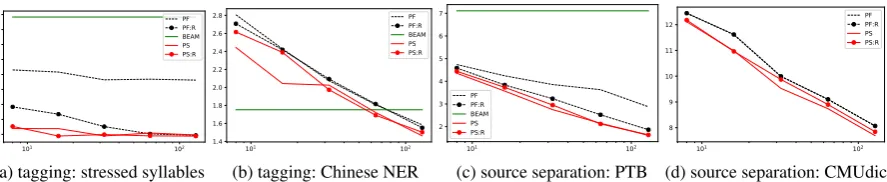
We now show that our proposed neural particle smoothing sampler does better than the particle filter-ing sampler. To define “better,” we evaluate samplers on theoffset KL divergencefrom the true posterior.

7.1 Evaluation metrics

Givenx, the “natural” goal of conditional sampling is for the sample distributionpˆ(y)to approximate the true distributionpθ(y|x) = expGT/expH0

from (1). We will therefore report—averaged over all held-out test examplesx—the KL divergence

KL(ˆp_||p) =Ey∼pˆ[log ˆp(y)] (34)

−(Ey∼pˆ[log ˜p(y|x)]−logZ(x)),

wherep˜(y|x)denotes theunnormalized distribu-tion given byexpGT in (2), andZ(x)denotes its

normalizing constant,expH0 =Pyp˜(y|x). As we are unable to computelogZ(x)in practice, we replace it with an estimate z(x) to obtain an offset KL divergence. This change of constant does not change the measured difference between two samplers, KL(ˆp1||p)−KL(ˆp2||p). Nonetheless, we

try to use a reasonable estimate so that the reported KL divergence is interpretable in an absolute sense. Specifically, we takez(x) = logP_y∈Yp˜(y|x)≤

logZ, where_Y is the full set of distinct particles ythat we ever drew for inputx, including samples from the beam search models, while constructing the experimental results graph.16 _{Thus, the offset}

KL divergence is a “best effort” lower bound on the true exclusive KL divergence KL(ˆp||p).

7.2 Results

In all experiments we compute the offset KL diver-gence for both the particle filtering samplers and the particle smoothing samplers, for varying ensemble sizesM. We also compare against a beam search

baseline that keeps the highest-scoringM particles

at each step (scored byexpGtwith no lookahead).

The results are in Figures2a–2d.

101 ₁₀2

0.25 0.50 0.75 1.00 1.25 1.50 1.75 2.00

2.25 _PF

PF:R BEAM PS PS:R

(a) tagging: stressed syllables

101 ₁₀2

1.4 1.6 1.8 2.0 2.2 2.4 2.6

2.8 PF

PF:R BEAM PS PS:R

(b) tagging: Chinese NER

101 ₁₀2

2 3 4 5 6 7

PF PF:R BEAM PS PS:R

(c) source separation: PTB

101 ₁₀2

8 9 10 11

12 PFPF:R

PS PS:R

(d) source separation: CMUdict

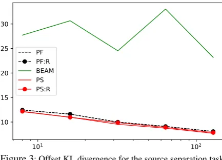
Figure 2: Offset KL divergences for the tasks in §§6.1and6.2. The logarithmicx-axis is the size of particlesM (8≤M _≤128). They-axis is the offset KL divergence described in§7.1(in bits per sequence). The smoothing samplers offer considerable speedup: for example, in Figure2a, the non-resampled smoothing sampler achieves comparable offset KL divergences with only1_{/4as many} particles as its filtering counterparts. Abbreviations in the legend: PF=particle filtering. PS=particle smoothing. BEAM=beam search. ‘:R’ suffixes indicate resampled variants. For readability, beam search results are omitted from Figure2d, but appear in Figure3of the appendices.

Given a fixed ensemble size, we see the smooth-ing sampler consistently performs better than the filtering counterpart. It often achieves comparable performance at a fraction of the ensemble size.

Beam search on the other hand falls behind on three tasks: stress prediction and the two source separation tasks. It does perform better than the stochastic methods on the Chinese NER task, but only at small beam sizes. Varying the beam size barely affects performance at all, across all tasks. This suggests that beam search is unable to explore the hypothesis space well.

We experiment with resampling for both the parti-cle filtering sampler and our smoothing sampler. In source separation and stressed syllable prediction, where the right context contains critical information about how viable a particle is, resampling helps par-ticle filteringalmostcatch up to particle smoothing. Particle smoothing itself is not further improved by resampling, presumably because its effective sam-ple size is high. The goal of resampling is to kill off low-weight particles (which were overproposed) and reallocate their resources to higher-weight ones. But with particle smoothing, there are fewer low-weight particles, so the benefit of resampling may be outweighted by its cost (namely, increased variance).

8 Related Work

Much previous work has employed sequential im-portance sampling for approximate inference of in-tractable distributions (e.g.,Thrun,2000;Andrews et al., 2017). Some of this work learns adaptive proposal distributions in this setting (e.g.Gu et al.,

2015;Paige and Wood,2016). The key difference in our work is that we consider future inputs, which is impossible in online decision settings such as robotics.Klaas et al.(2006) did do particle smooth-ing, like us, but they did not learn adaptive proposal distributions.

Just as we use a right-to-left RNN to guide pos-terior samplingof a left-to-right generative model,

Krishnan et al.(2017) employed a right-to-left RNN to guideposterior marginal inferencein the same sort of model.Serdyuk et al.(2018) used a right-to-left RNN to regularize training of such a model.

9 Conclusion

We have described neural particle smoothing, a se-quential Monte Carlo method for approximate sam-pling from the posterior of incremental neural scor-ing models. Sequential importance samplscor-ing has arguably been underused in the natural language pro-cessing community. It is quite a plausible strategy for dealing with rich, globally normalized probabil-ity models such as neural models—particularly if a good sequential proposal distribution can be found. Our contribution is a neural proposal distribution, which goes beyond particle filtering in that it uses a right-to-left recurrent neural network to “look ahead” to future symbols ofxwhen proposing each symbol yt. The form of our distribution is well-motivated.

There are many possible extensions to the work in this paper. For example, we can learn the generative model and proposal distribution jointly; we can also infuse them with hand-crafted structure, or use more deeply stacked architectures; and we can try training the proposal distribution end-to-end (footnote10). Another possible extension would be to allow each step ofqto propose asequenceof actions, effectively

making the tagset size∞. This extension relaxes our

|y|=|x|restriction from§1and would allow us to do general sequence-to-sequence transduction.

Acknowledgements

References

Roee Aharoni and Yoav Goldberg. 2017. Morphological inflection generation with hard monotonic attention. InACL.

Daniel Andor, Chris Alberti, David Weiss, Aliaksei Severyn, Alessandro Presta, Kuzman Ganchev, Slav Petrov, and Michael Collins. 2016.Globally normal-ized transition-based neural networks. InACL.

Nicholas Andrews, Mark Dredze, Benjamin Van Durme, and Jason Eisner. 2017. Bayesian modeling of lexical resources for low-resource settings. InACL.

Dzmitry Bahdanau, Philemon Brakel, Kelvin Xu, Anirudh Goyal, Ryan Lowe, Joelle Pineau, Aaron Courville, and Yoshua Bengio. 2017. An actor-critic algorithm for sequence prediction. InICLR.

Dzmitry Bahdanau, Kyunghyun Cho, and Yoshua Bengio. 2015. Neural machine translation by jointly learning to align and translate. InICLR.

Yoshua Bengio and Paolo Frasconi. 1996.Input-output HMMs for sequence processing.IEEE Transactions on Neural Networks, 7(5):1231–1249.

Bernhard E. Boser, Isabelle M. Guyon, and Vladimir N. Vapnik. 1992.A training algorithm for optimal margin classifiers. InCOLT.

Alexandre Bouchard-Côté, Percy Liang, Thomas Grif-fiths, and Dan Klein. 2007.A probabilistic approach to diachronic phonology. InEMNLP-CoNLL, pages 887–896.

Kyunghyun Cho, Bart van Merrienboer, Çaglar Gülçehre, Fethi Bougares, Holger Schwenk, and Yoshua Bengio. 2014. Learning phrase representations using RNN encoder-decoder for statistical machine translation. In EMNLP.

Ryan Cotterell, John Sylak-Glassman, and Christo Kirov. 2017.Neural graphical models over strings for prin-cipal parts morphological paradigm completion. In Proceedings of the 15th Conference of the European Chapter of the Association for Computational Linguis-tics: Volume 2, Short Papers, pages 759–765.

Randal Douc and Olivier Cappé. 2005.Comparison of resampling schemes for particle filtering. InImage and Signal Processing and Analysis, 2005. ISPA 2005. Proceedings of the 4th International Symposium on, pages 64–69. IEEE.

Arnaud Doucet and Adam M. Johansen. 2009.A tutorial on particle filtering and smoothing: Fifteen years later. Handbook of Nonlinear Filtering, 12(656-704):3.

Markus Dreyer and Jason Eisner. 2009.Graphical mod-els over multiple strings. InEMNLP.

Markus Dreyer, Jason R. Smith, and Jason Eisner. 2008.

Latent-variable modeling of string transductions with finite-state methods. InEMNLP.

Chris Dyer, Miguel Ballesteros, Wang Ling, Austin Matthews, and Noah A. Smith. 2015. Transition-based dependency parsing with stack long short-term memory. InACL.

Chris Dyer, Adhiguna Kuncoro, Miguel Ballesteros, and Noah A. Smith. 2016. Recurrent neural network gram-mars. InHLT-NAACL.

Jenny Rose Finkel, Christopher D. Manning, and An-drew Y. Ng. 2006.Solving the problem of cascading errors: Approximate Bayesian inference for linguistic annotation pipelines. InEMNLP.

Peter W. Glynn. 1990.Likelihood ratio gradient estima-tion for stochastic systems. Communications of the ACM, 33(10):75–84.

Shixiang Gu, Zoubin Ghahramani, and Richard E. Turner. 2015. Neural adaptive sequential Monte Carlo. In NIPS.

Peter E. Hart, Nils J. Nilsson, and Bertram Raphael. 1968.

A formal basis for the heuristic determination of mini-mal cost paths. 4(2):100–107.

Bruce Hayes. 1995.Metrical Stress Theory: Principles and Case Studies. University of Chicago Press.

Alexander T. Ihler and David A. McAllester. 2009. Parti-cle belief propagation. InAISTATS.

Eric Jang, Shixiang Gu, and Ben Poole. 2017. Cate-gorical reparameterization with Gumbel-softmax. In ICLR.

Katharina Kann and Hinrich Schütze. 2016. Single-model encoder-decoder with explicit morphological representation for reinflection. InACL.

Diederik P. Kingma and Jimmy Ba. 2015. Adam: A method for stochastic optimization. InICLR.

Mike Klaas, Mark Briers, Nando de Freitas, Arnaud Doucet, Simon Maskell, and Dustin Lang. 2006.Fast particle smoothing: If I had a million particles. In ICML.

Bjarne Knudsen and Michael M. Miyamoto. 2003. Se-quence alignments and pair hidden Markov models using evolutionary history.Journal of Molecular Bio-logy, 333(2):453 – 460.

Rahul G. Krishnan, Uri Shalit, and David Sontag. 2017.

Structured inference networks for nonlinear state space models. InAAAI.

John Lafferty, Andrew McCallum, and Fernando C. N. Pereira. 2001. Conditional random fields: Probabilis-tic models for segmenting and labeling sequence data. InICML.

Roderick J. A. Little and Donald B. Rubin. 1987. Sta-tistical Analysis with Missing Data. J. Wiley & Sons, New York.

Chris J. Maddison, Andriy Mnih, and Yee Whye Teh. 2017. The concrete distribution: A continuous relax-ation of discrete random variables. InICLR.

Mitchell P. Marcus, Mary Ann Marcinkiewicz, and Beat-rice Santorini. 1993. Building a large annotated cor-pus of English: The Penn treebank. Computational Linguistics, 19(2):313–330.

Andrew McCallum, Dayne Freitag, and Fernando Pereira. 2000. Maximum entropy Markov models for informa-tion extracinforma-tion and segmentainforma-tion. InMachine Learn-ing: Proceedings of the 17th International Conference (ICML 2000), pages 591–598, Stanford, CA.

Tomas Mikolov, Martin Karafiát, Lukas Burget, Jan Cer-nock`y, and Sanjeev Khudanpur. 2010. Recurrent neu-ral network based language model. InInterspeech, volume 2, page 3.

Brooks Paige and Frank D. Wood. 2016. Inference net-works for sequential Monte Carlo in graphical models. InICML.

Brooks Paige, Frank D. Wood, Arnaud Doucet, and Yee Whye Teh. 2014. Asynchronous anytime sequen-tial Monte Carlo. InNIPS.

Nanyun Peng and Mark Dredze. 2015. Named en-tity recognition for Chinese social media with jointly trained embeddings. InEMNLP.

Jeffrey Pennington, Richard Socher, and Christopher D. Manning. 2014. GloVe: Global vectors for word rep-resentation. InEMNLP.

Fernando C. N. Pereira and Michael D. Riley. 1997.

Speech recognition by composition of weighted finite automata. Finite-State Language Processing, page 431.

Lawrence R. Rabiner. 1989.A tutorial on hidden Markov models and selected applications in speech recognition. Proceedings of IEEE, 77(2):257–285.

Lance A. Ramshaw and Mitchell P. Marcus. 1999. Text chunking using transformation-based learning. In Na-tural Language Processing Using Very Large Corpora, pages 157–176. Springer.

Branko Ristic, Sanjeev Arulampalam, and Neil James Gordon. 2004. Beyond the Kalman Filter: Particle Filters for Tracking Applications. Artech House.

Herbert Robbins and Sutton Monro. 1951.A stochastic approximation method. The Annals of Mathematical Statistics, pages 400–407.

Dmitriy Serdyuk, Nan Rosemary Ke, Alessandro Sordoni, Adam Trischler, Chris Pal, and Yoshua Bengio. 2018.

Twin networks: Matching the future for sequence ge-neration. InICLR.

Andreas Stuhlmüller, Jacob Taylor, and Noah Goodman. 2013.Learning stochastic inverses. InNIPS.

Sebastian Thrun. 2000.Monte Carlo POMDPs. InNIPS.

Andrew J. Viterbi. 1967.Error bounds for convolutional codes and an asymptotically optimum decoding al-gorithm. IEEE Transactions on Information Theory, IT-13(2):260–269.

Greg C. G. Wei and Martin A. Tanner. 1990.A Monte Carlo implementation of the EM algorithm and the poor man’s data augmentation algorithms. Journal of the American Statistical Association, 85(411):699– 704.

Robert L. Weide. 1998. The CMU pronunciation dictio-nary, release 0.6.

Ronald J. Williams. 1992. Simple statistical gradient-following algorithms for connectionist reinforcement learning.Machine Learning, 8(23).

Sam Wiseman and Alexander M. Rush. 2016. Sequence-to-sequence learning as beam-search optimization. In EMNLP.

Hiroyasu Yamada and Yuji Matsumoto. 2003.Statistical dependency analysis with support vector machines. In Proceedings of IWPT, volume 3, pages 195–206.

Michael Zibulevsky and Barak A. Pearlmutter. 2001.

A The logprob-to-go for HMMs

As noted in§2.1, the logprob-to-goHtcan be

com-puted by the backward algorithm. By the definition ofHtin equation (10),

expHt= X

yt:

exp (GT −Gt) (35)

=X

y_t: exp

T X

j=t+1

gθ(sj−1, xj, yj) (36)

=X

y_t:

T Y

j=t+1

pθ(yj |yj−1)·pθ(xj |yj)

= (β_t)yt (backward prob ofytat timet)

where the vectorβ_tis defined by base case(β_T)y =

1and for0_≤t < T by the recurrence

(βt)y =def X

yt:

pθ(xt:,yt:|yt=y) (37)

=X

y0

pθ(y0 |y)·pθ(xt+1 |y0)·(βt+1)y0

The backward algorithm (20) for OOHMMs in

§2.2is a variant of this.

B Gradients for Training the Proposal Distribution

For a givenx, both forms of KL divergence achieve

their minimum of 0 when(_∀y)qφ(y|x) =p(y|

x). However, we are unlikely to be able to find such

aφ; the two metrics penalizeqφdifferently for

mis-matches. We simplify the notation below by writing

qφ(y)andp(y), suppressing the conditioning onx.

Inclusive KL Divergence The inclusive KL di-vergence has that name because it is finite only when support(qφ)⊇support(p), i.e., whenqφis capable

of proposing any stringythat has positive proba-bility underp. This is required forqφto be a valid

proposal distribution for importance sampling.

KL(p||qφ) (38)

=Ey∼p[logp(y)−logqφ(y)]

=_Ey∼p[logp(y)]

−Ey∼p[logqφ(y)]

The first termEy∼p[logp(y)]is a constant with

regard toφ. As a result, the gradient of the above is just the gradient of the second term:

∇φKL(p||qφ) =∇φEy∼p[−logqφ(y)]

| {z }

the cross-entropyH(p,qφ)

We cannot directly sample from p. However, our weighted mixturepˆfrom equation (28) (obtained by sequential importance sampling) could be a good approximation:

∇φKL(p||qφ)≈ ∇φEy∼pˆ[−logqφ(y)] (39)

=

T X

t=1

Epˆ[−∇φlogqφ(yt|y:t−1,x)]

Following this approximate gradient downhill has an intuitive interpretation: if a particularytvalue ends

up with high relative weight in the final ensemblepˆ, then we will try to adjustqφso that it would have

had a high probability of proposing thatytvalue at

steptin the first place.

Exclusive KL Divergence The exclusive diver-gence has that name because it is finite only when support(qφ)⊆support(p). It is defined by

KL(qφ||p) =Ey∼qφ[logqφ(y)−logp(y)] (40)

=Ey∼qφ[logqφ(y)−log ˜p(y)] + logZ

=X

y

qφ(y) [logqφ(y)−log ˜p(y)]

| {z }

call thisdφ(y)

+ logZ

where_P p(y) = _Z1p˜(y)forp˜(y) = expGT andZ =

yp˜(y). With some rearrangement, we can write its gradient as an expectation that can be estimated by sampling fromqφ.17Observing thatZis constant

with respect toφ, first write

∇φKL(qφ||p) (41)

=X

y

∇φ(qφ(y)dφ(y)) (42)

=X

y

(∇φqφ(y))dφ(y)

+X

y

qφ(y)∇φlogqφ(y)

| {z }

=∇φqφ(y)

=X

y

(_∇φqφ(y))dφ(y)

where the last step uses the fact that_P y∇φqφ(y) = ∇φPyqφ(y) = ∇φ1 = 0.

We can turn this into an expectation with a second use of Glynn (1990)’s observation that

17_{This is an extension of the REINFORCE trick (Williams,}

∇φqφ(y) = qφ(y)∇φlogqφ(y) (the “likelihood

ratio trick”):

∇φKL(qφ||p)

=X

y

qφ(y)dφ(y)∇φlogqφ(y)

=Ey∼qφ[dφ(y)∇φlogqφ(y)] (43)

which can, if desired, be further rewritten as =_Ey∼qφ[dφ(y)∇φdφ(y)]

=Ey∼qφ

∇φ 1₂dφ(y)2 (44)

If we regarddφ(y)as a signed error (in the log

do-main) in trying to fitqφtop˜, then the above gradient

of KL can be interpreted as the gradient of the mean squared error (divided by 2).18

We would get the same gradient for any rescaled version of the unnormalized distributionp˜, but the formula for obtaining that gradient would be dif-ferent. In particular, if we rewrite the above deriva-tion but add a constantbto bothlog ˜p(y)andlogZ

throughout (equivalent to addingbtoGT), we will

get the slightly generalized expectation formulas

Ey∼qφ[(dφ(y)−b)∇φlogqφ(y)] (45) Ey∼qφ

h

∇φ

1

2(dφ(y)−b)

2i ₍₄₆₎

in place of equations (43) and (44). By choosing an appropriate “baseline”b, we can reduce the variance

of the sampling-based estimate of these expectations. This is similar to the use of a baseline in the REIN-FORCE algorithm (Williams,1992). In this work we choosebusing an exponential moving average of pastE[dφ(y)]values: at the end of each training

minibatch, we updateb_←0.1_·b+ 0.9_·d¯, where

¯

dis the mean of the estimatedEy∼qφ(·|x)[dφ(y)]

values for all examplesxin the minibatch. C Implementation Details

We implement all RNNs in this paper as GRU net-works (Cho et al.,2014) withd= 32hidden units (state spaceR32_{). Each of our models (§6) always}

specifies the logprob-so-far in equations (2) and (3) using a 1-layer left-to-right GRU,19_{while the}

corre-sponding proposal distribution (§3.3) always spec-ifies the statestin (6) using a 2-layer right-to-left

18_{We thank Hongyuan Mei, Tim Vieira, and Sanjeev} Khu-danpur for insightful discussions on this derivation.

19_{For the tagging task described in§6.1,g}

θ(st−1, xt, yt)def=

logpθ(xt, yt | st−1), where the GRU statest−1 is used to define a softmax distribution over possible(xt, yt)pairs in the

same manner as an RNN language model (Mikolov et al.,2010). Likewise, for the source separation task (§6.2), the source lan-guage models described in AppendixGare GRU-based RNN language models.

101 ₁₀2

10 15 20 25 30

PF PF:R BEAM PS PS:R

Figure 3: Offset KL divergence for the source separation task on phoneme sequences.

GRU, and specifies the compatibility functionCtin

(23) using a4-layer feedforward ReLU network.20

For the Chinese social media NER task (§6.1), we use the Chinese character embeddings provided by

Peng and Dredze(2015), while for the source separa-tion tasks (§6.2), we use the 50-dimensional GloVe word embeddings (Pennington et al.,2014). In other cases, we train embeddings along with the rest of the network. We optimize with the Adam optimizer using the default parameters (Kingma and Ba,2015) andL2regularization coefficient of10−5.

D Training Procedures

In all our experiments, we train the incremental scor-ing models (the taggscor-ing and source separation mod-els described in§6.1and§6.2, respectively) on the training datasetT. We do early stopping, using

per-plexity on a held-out development setD1to choose

the number of epochs to train (maximum of3). Having obtained these model parametersθ, we

train our proposal distributionsqθ,φonT, keeping

θfixed and only tuningφ. Again we use early

stop-ping, using the KL divergence from§7.1on a sep-arate development setD2to choose the number of

epochs to train (maximum of20 for the two tag-ging tasks and source separation on the PTB dataset, and maximum of50 for source separation on the phoneme sequence dataset). We then evaluateqθ∗_,φ∗

on the test datasetE.

[AppendicesE–Gappear in the supplementary material file.]

20_{As input toC}

t, we actually provide not onlyst,¯stbut also

the statesfθ(st−1, xt, y)(includingst) that could have been

reached foreachpossible valueyofyt. We have to compute