High-Performance, Language-Independent Morphological Segmentation
Sajib Dasgupta
and
Vincent Ng
Human Language Technology Research Institute
University of Texas at Dallas
Richardson, TX 75083-0688
{sajib,vince}@hlt.utdallas.edu
Abstract
This paper introduces an unsupervised morphological segmentation algorithm that shows robust performance for four languages with different levels of mor-phological complexity. In particular, our algorithm outperforms Goldsmith’s Lin-guistica and Creutz and Lagus’s Mor-phessor for English and Bengali, and achieves performance that is comparable to the best results for all three PASCAL evaluation datasets. Improvements arise from (1) the use of relative corpus fre-quency and suffix level similarity for de-tecting incorrect morpheme attachments and (2) the induction of orthographic rules and allomorphs for segmenting words where roots exhibit spelling changes dur-ing morpheme attachments.
1
Introduction
Morphological analysis is the task of segmenting a word into morphemes, the smallest
meaning-bearing elements of natural languages. Though very successful, knowledge-based morphological
analyzers operate by relying on manually designed segmentation heuristics (e.g. Koskenniemi (1983)), which require a lot of linguistic expertise and are time-consuming to construct. As a result, research in morphological analysis has exhibited a shift to
unsupervised approaches, in which a word is
typi-cally segmented based on morphemes that are automatically induced from an unannotated corpus. Unsupervised approaches have achieved
consider-able success for English and many European lan-guages (e.g. Goldsmith (2001), Schone and Juraf-sky (2001), Freitag (2005)). The recent PASCAL Challenge on Unsupervised Segmentation of Words into Morphemes1 has further intensified
interest in this problem, selecting as target lan-guages English as well as two highly agglutinative languages, Turkish and Finnish. However, the evaluation of the Challenge reveals that (1) the success of existing unsupervised morphological parsers does not carry over to the two agglutinative languages, and (2) no segmentation algorithm achieves good performance for all three languages.
Motivated by these state-of-the-art results, our goal in this paper is to develop an unsupervised
morphological segmentation algorithm that can
work well across different languages. With this
goal in mind, we evaluate our algorithm on four languages with different levels of morphological complexity, namely English, Turkish, Finnish and Bengali. It is worth noting that Bengali is an under-investigated Indo-Aryan language that is highly inflectional and lies between English and Turk-ish/Finnish in terms of morphological complexity. Experimental results demonstrate the robustness of our algorithm across languages: it not only outper-forms Goldsmith’s (2001) Linguistica and Creutz and Lagus’s (2005) Morphessor for English and Bengali, but also compares favorably to the best-performing PASCAL morphological parsers when evaluated on all three datasets in the Challenge.
The performance improvements of our segmen-tation algorithm over existing morphological ana-lyzers can be attributed to our extending Keshava and Pitler’s (2006) segmentation method, the best performer for English in the aforementioned
PASCAL Challenge, with the capability of han-dling two under-investigated problems:
Detecting incorrect attachments. Many existing
morphological parsers incorrectly segment “candi-date” as “candid”+“ate”, since they fail to identify that the morpheme “ate” should not attach to the
word “candid”. Schone and Jurafsky’s (2001) work represents one of the few attempts to address this inappropriate morpheme attachment problem, in-troducing a method that exploits the semantic re-latedness between word pairs. In contrast, we propose two arguably simpler, yet effective tech-niques that rely on relative corpus frequency and suffix level similarity to solve the problem.
Inducing orthographic rules and allomorphs.
One problem with Keshava and Pitler’s algorithm is that it fails to segment words where the roots exhibit spelling changes during attachment to mor-phemes (e.g. “denial” = “deny”+“al”). To address this problem, we automatically acquire allomorphs and orthographic change rules from an unannotated corpus. These rules also allow us to output the ac-tual segmentation of the words that exhibit spelling changes during morpheme attachment, thus avoid-ing the segmentation of “denial” as “deni”+”al”, as is typically done in existing morphological parsers. In addition to addressing the aforementioned problems, our segmentation algorithm has two ap-pealing features. First, it can segment words with any number of morphemes, whereas many analyz-ers can only be applied to words with one root and one suffix (e.g. DéJean (1998), Snover and Brent (2001)). Second, it exhibits robust performance even when inducing morphemes from a very large vocabulary, whereas Goldsmith’s (2001) and Freitag’s (2005) morphological analyzers perform well only when a small vocabulary is employed, showing deteriorating performance as the vocabu-lary size increases.
The rest of this paper is organized as follows. Section 2 presents related work on unsupervised morphological analysis. In Section 3, we describe our basic morpheme induction algorithm. We then show how to exploit the induced morphemes to (1) detect incorrect attachments by using relative cor-pus frequency (Section 4) and suffix level similar-ity (Section 5) and (2) induce orthographic rules and allomorphs (Section 6). Section 7 describes our algorithm for segmenting a word using the in-duced morphemes. We present evaluation results in Section 8 and conclude in Section 9.
2
Related Work
As mentioned in the introduction, the problem of unsupervised morphological learning has been ex-tensively studied for English and many other European languages. In this section, we will give an overview of the related work on this problem.
Harris (1955) develops a strategy for identifying morpheme boundaries that checks whether the number of different letters following a sequence of letters exceeds some given threshold. DéJean (1998) improves Harris’s segmentation algorithm by first inducing a list of 100 most frequent mor-phemes and then using those mormor-phemes for word segmentation. The aforementioned PASCAL Chal-lenge on Unsupervised Word Segmentation has undoubtedly intensified interest in this problem. Among the participating groups, Keshava and Pit-ler’s (2006) segmentation algorithm combines the ideas of DéJean and Harris and achieves the best result for the English dataset, but it only offers me-diocre performance for Finnish and Turkish.
There is another class of unsupervised morpho-logical learning algorithms whose design is driven by the Minimum Description Length (MDL) prin-ciple. Specifically, EM is used to iteratively seg-ment a list of words using some predefined heuristics until the length of the morphological grammar converges to a minimum. Brent et al. (1995) are the first to introduce an information-theoretic notion of compression to represent the MDL framework. Goldsmith (2001) also adopts the MDL approach, providing a new compression system that incorporates signatures when measur-ing the length of the morphological grammar. Creutz (2003) proposes a probabilistic maximum a posteriori formulation that uses prior distributions
of morpheme length and frequency to measure the goodness of an induced morpheme, achieving bet-ter results for Finnish but worse results for English in comparison to Goldsmith’s Linguistica.
3
The Basic Morpheme Induction
Algo-rithm
Our unsupervised segmentation algorithm is com-posed of two steps: (1) inducing prefixes, suffixes
and roots from a vocabulary that consists of words
3.1
Extracting a List of Candidate AffixesThe first step of our morpheme induction method involves extracting a list of candidate prefixes and suffixes. We rely on a fairly simple idea originally proposed by Keshava and Pitler (2006) for extract-ing candidate affixes. Assume that and
are two character sequences and
is the concatenation of and
. If
and are both found in the vocabu-lary, then we extract
as a candidate suffix. Simi-larly, if
and
are both found in the vocabulary, then we extract as a candidate prefix.
The above affix induction method is arguably overly simplistic and therefore can generate many spurious affixes. To filter spurious affixes, we (1) score each affix by multiplying its frequency (i.e.
the number of distinct words to which each affix attaches) and its length2, and then (2) retain only
the K top-scoring affixes, where K is set differently
for prefixes and suffixes. The value of K is
some-what dependent on the vocabulary size, as the af-fixes in a larger vocabulary system are generated from a larger number of words. For example, we set the thresholds to 70 for prefixes and 50 for suf-fixes for English; on the other hand, since the Fin-nish vocabulary is almost six times larger than that of English, we set the corresponding thresholds to be approximately six times larger (400 and 300 for prefixes and suffixes respectively).3
3.2
Detecting Composite SuffixesNext, we detect and remove composite suffixes (i.e.
suffixes that are formed by combining multiple suffixes [e.g. “ers” = “er”+“s”]) from our induced suffix list, because their presence can lead to un-der-segmentation of words (e.g. “walkers”, whose correct segmentation is “walk”+“er”+“s”, will be erroneously segmented as “walk”+“ers”). Compos-ite suffix detection is a particularly important prob-lem for languages like Bengali in which composite suffixes are abundant (see Dasgupta and Ng (2007)). Note, however, that simple concatenation of multiple suffixes does not always produce a composite suffix. For example, “ent”, “en” and “t” all are valid suffixes in English, but “ent” is not a
2 The dependence on frequency and length is motivated by the observation that
less-frequent and shorter affixes (especially those of length 1) are more likely to be erroneous (see Goldsmith (2001)).
3 Since this method for setting our vocabulary-dependent thresholds is fairly
simple, the use of these thresholds should not be viewed as rendering our seg-mentation algorithm language-dependent.
composite suffix. Hence, we need a more sophisti-cated method for composite suffix detection.
Our detection method is motivated by the fol-lowing observation: if xy is a composite suffix and
a word w combines with xy, then it is highly likely
that w will also combine with its first component
suffix x. Note that this property does not hold for
non-composite suffixes. For instance, words that combine with the non-composite suffix “ent” (e.g. “absorb”) do not combine with its first component suffix “en”. Consequently, given two suffixes x
and y, our method posits xy as a composite suffix if xy and x are similar in terms of the words to which
they attach. Specifically, we consider xy and x to
be similar if their similarity value as computed by the formula below is greater than 0.6:
| |
|' | ) | ( ) , (
W W xy x P x xy
Similarity = = ,
where |W| is the number of distinct words that
combine with both xy and x, and |W| is the number
of distinct words that combine with xy.
3.3
Extracting a List of Candidate RootsFinally, we extract a list of candidate roots using the induced list of affixes as follows. For each word, w, in the vocabulary, we check whether w is divisible, i.e. whether w can be segmented as r+x
or p+r, where p is an induced prefix, x is an
in-duced suffix, and r is a word in the vocabulary. We
then add w to the root list if it is not divisible.
Note, however, that the resulting root list may con-tain compound words (i.e. words with multiple
roots). Hence, we make another pass over our root list to remove any word that is a concatenation of multiple words in the vocabulary.
4
Detecting Incorrect Attachments Using
Relative Frequency
cor-pus frequency to determine whether the attachment of a morpheme to a root word is plausible or not.
Consider again the two words “candidate” and “candid”. While “candidate” occurs 6380 times in our corpus, “candid” occurs only 119 times. This frequency disparity can be an important clue to determining that there is no morphological relation between “candidate” and “candid”. Similar obser-vation is also made by Yarowsky and Wicentowski (2000), who successfully employ relative fre-quency similarity or disparity to rank candidate VBD/VB pairs (e.g. “sang”/“sing”) that are irregu-lar in nature. Unlike Yarowsky and Wicentowski, however, our goal is to detect incorrect affix at-tachments and improve morphological analysis.
Our incorrect attachment detection algorithm, which exploits frequency disparity, is based on the following hypothesis: if a word w is formed by
attaching an affix m to a root word r, then the
cor-pus frequency of w is likely to be less than that of r
(i.e. the frequency ratio of w to r is less than one).
In other words, we hypothesize that the inflectional or derivational forms of a root word occur less fre-quently in a corpus than the root itself.
To illustrate this hypothesis, Table 1 shows some randomly chosen English words together with their word-root frequency ratios (WRFRs).
The <word, root> pairs in the left side of the table are examples of correct attachments, whereas those in the right side are not. Note that only those words that represent correct attachments have a WRFR less than 1.
The question, then, is: to what extent does our hypothesis hold? To investigate this question, we generated examples of correct attachments by ran-domly selecting 400 words from our English vo-cabulary and then removing those that are root words, proper nouns, or compound words. We then manually segmented each of the remaining 378 words as Prefix+Root or Root+Suffix with the aid of the CELEX lexical database (Baayean et al., 1996). Somewhat surprisingly, we found that the WRFR is less than 1 in only 71.7% of these at-tachments. When the same experiment was re-peated on 287 hand-segmented Bengali words, the hypothesis achieves a higher accuracy of 83.6%.
To better understand why our hypothesis does not work well for English, we measured its accu-racy separately for the Root+Suffix words and the Prefix+Root words, and found that the hypothesis fails mostly on the suffixal attachments (see Table
2). Though surprising at first glance, the relatively poor accuracy on suffixal attachments can be at-tributed to the fact that many words in English (e.g. “amusement”, “winner”) appear more fre-quently in our corpus than their corresponding root forms (e.g. “amuse”, “win”). For Bengali, our hy-pothesis fails mainly on verbs, whose inflected forms occur more often in our corpus than their roots. This violation of the hypothesis can be at-tributed to the grammatical rule that the main verb of a Bengali sentence has to be inflected according to the subject in order to maintain sentence order.
To improve the accuracy of our hypothesis on detecting correct attachments, we relax our initial hypothesis as follows: if an attachment is correct, then the corresponding WRFR is less than some predefined threshold t, where t > 1. However, we
do not want t to be too large, since our algorithm
may then determine many incorrect attachments as correct. In addition, since our hypothesis has a high accuracy for prefixal attachments than suffixal at-tachments, the threshold we employ for prefixes can be smaller than that for suffixes. Taking into account these considerations, we use a threshold of 10 for suffixes and 2 for prefixes for all the lan-guages we consider in this paper.
Correct Parses Incorrect Parses
Word Root WRFR Word Root WRFR
bear-able bear 0.01 candid-ate candid 53.6 attend-ance attend 0.24 medic-al medic 483.9 arrest-ing arrest 0.06 prim-ary prim 327.4 sub-group group 0.0002 ac-cord cord 24.0 re-cycle cycle 0.028 ad-diction diction 52.7 un-settle settle 0.018 de-crease crease 20.7
Table 1: Word-root frequency ratios
Root+Suffix Prefix+Root Overall
# of words 344 34 378
WRFR < 1 70.1% 88.2% 71.7%
Table 2:Hypothesis validation for English Now we can employ our hypothesis to detect in-correct attachments and improve root induction as follows. For each word, w, in the vocabulary, we
check whether (1) w can be segmented as r+x or p+r, where p and x are valid prefixes and suffixes
respectively and r is another word in the
vocabu-lary, and (2) the WRFR for w and r is less than our
predefined thresholds (10 for suffixes and 2 for prefixes). If both conditions are satisfied, it means that w is divisible.Hence, we add w into the list of
5
Suffix Level Similarity
Many of the incorrect suffixal attachments have a WRFR between 1 and 10, but the detection algo-rithm described in the previous section will deter-mine all of them as correct attachments. Hence, in this section, we propose another technique, which we call suffix level similarity, to identify some of
these incorrect attachments.
Suffix level similarity is motivated by the fol-lowing observation: if a word w combines with a
suffix x, then w should also combine with the
suf-fixes that are “morphologically similar” to x. To
exemplify, consider the suffix “ate” and the root word “candid”. The words that combine with the suffix “ate” (e.g. “alien”, “fabric”, “origin”) also combine with suffixes like “ated”, “ation” and “s”. Given this observation, the question of whether “candid” combines with the suffix “ate” then lies in whether or not “candid” combines with “ated”, “s” and “ation”. The fact that “candid” does not combine with many of the above suffixes provides suggestive evidence that “candidate” cannot be derived from “candid”.
More specifically, to check whether a word w
combines with a suffix x using suffix level
simial-rity, we (1) find the set of words Wx that can com-bine with x; (2) find the set of suffixes Sx that attach to all of the words in Wx under the constraint that Sx does not contain x; and (3) find the 10 suf-fixes in Sx that are most “similar” to x. The
ques-tion, then, is how to define similarity. Intuitively, a good similarity metric should reflect, for instance, the fact that “ated” is a better suffix to consider in the attachment decision for “ate” than “s” (i.e. “ated” is more similar to “ate” than “s”), since “s” attaches to most nouns and verbs in English and hence should not be a distinguishing feature for incorrect attachment detection.
We employ a probabilistic measure (PM) that computes the similarity between suffixes x and y as
the product of (1) the probability of a word com-bining with y given that it combines with x and (2)
the probability of a word combining with x given
that it combines with y. More specifically,
, * ) | ( * ) | ( ) , (
2
1 n
n n
n y x P x y P y x
PM = =
where n1 is the number of distinct words that com-bine with x, n2 is the number of distinct words that
combine with y, and n is the number of distinct
words that combine with both x and y.4
After getting the 10 suffixes that are most simi-lar to x, we employ them as features and use the
associated similarity values (we scale them linearly between 1 and 10) as the weights of these 10 fea-tures. The decision of whether a suffix x can attach
to a word w depends on whether the following
ine-quality is satisfied:
,
10
1
t w fi i >
where fi is a boolean variable that has the value 1 if
w combines with xi, where xi is one of the 10 suf-fixes that are most similar to x; wi is the scaled similarity between x and xi; and t is a predefined
threshold that is greater than 0.
One potential problem with suffix level similar-ity is that it is an overly strict condition for those words that combine with only one or two suffixes in the vocabulary. For example, if the word “char-acter” has just one variant in the vocabulary (e.g. “characters”), suffix level similarity will determine the attachment of “s” to “character” as incorrect, since the weighted sum in the above inequality will be 0. To address this sparseness problem, we rely on both relative corpus frequency and suffix level similarity to identify incorrect attachments. Spe-cifically, if the WRFR of a <word, root> pair is between 1 and 10, we determine that an attachment to the root is incorrect if
-WRFR + * (suffix level similarity) < 0,
where is set to 0.15.
Finally, since long words have a higher chance of getting segmented, we do not apply suffix level similarity to words whose length is greater than 10.
6
Inducing Orthographic Rules and
Al-lomorphs
The biggest drawback of the system, described thus far, is its failure to segment words where the roots exhibit spelling changes during attachment to morphemes (e.g. “denial” = “deny”+“al”). The reasons are (1) the system does not have any knowledge of language-specific orthographic rules (e.g. in English, the character ‘y’ at the morpheme boundary is changed to ‘i’ when the root combines
4 Note that this metric has the desirable property of returning a low similarity
with the suffix “al”), and (2) the vocabulary we employ for morpheme induction does not normally contain the allomorphic variations of the roots
(e.g. “deni” is allomorphic variation of “deny”). To segment these words correctly, we need to generate the allomorphs and orthographic rules automati-cally given a set of induced roots and affixes.
Before giving the details of the generation method, we note that the induction of orthographic rules is a challenging problem, since different lan-guages exhibit orthographic changes in different ways. For some languages (e.g. English) rules are mostly predictable, whereas for others (e.g. Fin-nish) rules are highly irregular. It is hard to obtain a generalized mapping function that aligns every <root, allomorph> pair, considering the fact that our system is unsupervised. An additional chal-lenge is to ensure that the incorporation of these orthographic rules will not adversely affect system performance (i.e. they will not be applied to regu-lar words and thus segment them incorrectly). Yarowsky and Wicentowski (2000) propose an interesting algorithm that employs four similarity measures to successfully identify the most prob-able root of a highly irregular word. Unlike them, however, our goal is to (1) check whether the learned rules can actually improve an unsupervised morphological system, not just to align <root, al-lomorph> pair, and (2) examine whether our sys-tem is extendable to different languages.
Taking into consideration the aforementioned challenges, our induction algorithm will (1) handle orthographic character changes that occur only at morpheme boundaries; (2) generate allomorphs for suffixal attachments only5, assuming that roots ex-hibit the character changes during attachment, not suffixes; and (3) learn rules that aligns <root, allo-morph> pairs of edit distance 1 (which may in-volve 1-character replacement, deletion or insertion). Despite these limitations, we will see that the incorporation of the induced rules im-proves segmentation accuracy significantly.
Let us first discuss how we learn a replacement
rule, which identifies <allomorph, root> pairs where the last character of the root is replaced by another character. The steps are as follows:
(1) Inducing candidate allomorphs
If A
is a word in the vocabulary (e.g. “denial”, where =“den”, A=“i”, and
=“al”),
is an
5 We only learn rules for suffixes of length greater than 1, since most suffixes of
length 1 do not participate in orthographic changes.
duced suffix, B is an induced root (e.g. “deny”,
where B=“y”), and the attachment of
to B is
correct according to relative corpus frequency (see Section 4), then we hypothesize that A is an
allo-morph of B. For each induced suffix, we use this
hypothesis to generate the allomorphs and identify those that are generated from at least two suffixes as candidate allomorphs. We denote the list of
<candidate allomorph, root, suffix> tuples by L.
(2) Learning orthographic rules
Every <candidate allomorph, root, suffix> tuple as learned above is associated with an orthographic rule. For example, from the words “denial”, “deny” and suffix “al”, we learn the rule “y:i / _ + al”6; from “social”, “sock” and “al”, we learn the rule “k:i / _ + al”, which, however, is erroneous. So, we check whether each of the learned rules occurs fre-quently enough for all the <allomorph, root> pairs associated with a suffix, with the goal of filtering the low-frequency orthographic rules. Specifically, for each suffix
, we repeat the following steps:
(a) Counting the frequency of rules. Let L be the
list of <candidate allomorph, root> pairs in L that
are associated with the suffix
. For each pair p in L, we first check whether its candidate allomorph
appears in any other <candidate allomorph, root> pairs in L . If not, we increment the frequency of
the orthographic rule associated with p by 1. For
example, the pair <“deni”, “deny”> increases the frequency of the rule “y:i” by 1 on condition that “deni” does not appear in any other pairs.
(b) Filtering the rules. We first remove the
infre-quent rules, specifically those that are induced by less than 15% of the tuples in L. Then we check
whether there exists two rules of the form A:B and A:C in the induced rule list. If so, then we have a
morphologically undesirable situation where the character A changes to B and C under the same
environment (i.e.
). To address this problem, we first calculate the strength of a rule as follows:
=
@
@) : (
) : ( )
: (
A frequency
B A frequency B
A strength
We then retain only those rules whose fre-quency*strength is greater than some predefined threshold. We denote the list of rules that satisfy the above constraints by R.
(c) Identifying valid allomorphs. For each rule in
R, we identify the associated <candidate
6 This is the Chomsky and Halle notation for representing orthographic rules. a:b
morph, root> pairs in L . We refer to the candidate
allomorphs in each of those pairs as valid allo-morphs and add them to the list of roots. We also
remove from the original root list the words that can be segmented by the induced allomorphs and the associated rules (e.g. “denial”).
(d) Identifying composite suffixes. For each rule
in R, we also check whether it can identify
com-posite suffixes where the first component suffix’s last character is replaced during attachment to the second component suffix (e.g. “liness” = “ly”+“ness”). Specifically, if (1) A:B / _
is a rule in R , (2) A
(say “liness”),
(say “ness”) and B
(say “ly”) are induced suffixes, and (3) A
satis-fies the requirements of a composite suffix (see Section 3.2), then we determine that A
is a com-posite suffix composed of B and
.
We employ the same procedure for learning in-sertion and deletion rules, except that strength is
always set to 1 for these two types of rules. The threshold we set at step (b) is somewhat dependent on the vocabulary size, since the frequency count of each rule will naturally be larger when a larger vocabulary is used. Following our method for set-ting vocabulary-dependent thresholds (see Section 3.1), we set the threshold to 4 for English and 25 for Finnish, for instance.
Finally, we adapt our candidate allomorph de-tection method described above to induce allo-morphs that are generated through orthographic changes of edit distance greater than 1. Specifi-cally, if
is a word in the induced root list (e.g. “stability”7, where =“stabil” and
=“ity”),
is an induced suffix, and the attachment of
to is cor-rect according to suffix level similarity, then we hypothesize that (“stabil”) is a candidate allo-morph. For each induced suffix, we use this hy-pothesis to generate candidate allomorphs and consider as valid allomorphs only those that are generated from at least three different suffixes.8
7
Word Segmentation
After inducing the morphemes, we can use them to segment a word w in the test set. Specifically, we
7 The correct segmentation of “stability” is “stable”+“ity”. The “stabil”-“stable”
allomorph-root pair is an example of an orthographic change of edit distance 2.
8 This technique can also be used to induce out-of-vocabulary (OOV) roots. For
example, the presence of “perplexity”, “perplexed” and “perplexing” in a vo-cabulary allows us to induce the root “perplex”. OOV root induction is particu-larly important for languages like Bengali, where verb roots mostly take the imperative form and hence are absent in a vocabulary created from a newspaper corpus, which normally comprises only the first and third person verb forms.
(1) generate all possible segmentations of w using
only the induced affixes and roots, and (2) apply a sequence of tests to remove candidate
segmenta-tions until we are left with only one candidate, which we take to be the final segmentation of w.
Our first test involves removing any candidate segmentation m1m2 … mn that violates any of the linguistic constraints below:
• At least one of m1, m2, …, mn is a root.
• For 1 ≤i < n, if mi is a prefix, then mi+1 must be a root or a prefix.
• For 1 < i≤n, if mi is a suffix, then mi-1 must be a root or a suffix.
• m1 can’t be a suffix and mn can’t be a prefix. Next, we apply our second test, in which we re-tain only those candidate segmentations that have the smallest number of morphemes. For example, if “friendly” has two candidate segmentations “friend”+“ly” and “fri”+“end”+“ly”, we will select the first one to be the segmentation of w.
If more than one candidate segmentation still ex-ists, we score each remaining candidate using the heuristic below, selecting the highest-scoring can-didate to be the final segmentation of w. Basically,
we score each candidate segmentation by adding the strength of each morpheme in the
segmenta-tion, where (1) the strength of an affix is the num-ber of distinct words in the vocabulary to which the affix attaches, multiplied by the length of the affix, and (2) the strength of a root is the number of distinct morphemes with which the root combines, again multiplied by the length of the root.
8
Evaluation
In this section, we will first evaluate our segmenta-tion algorithm for English and Bengali, and then examine its performance on the PASCAL datasets.
8.1
Experimental SetupVocabulary creation. We extracted our English
steps to five years of articles taken from the Ben-gali newspaper Prothom Alo to generate our
Ben-gali vocabulary, which consists of 140K words.
Test set preparation. To create our English test
set, we randomly chose 000 words from our vo-cabulary that are at least 4-character long9 and also appear in CELEX. Although 95% of the time we adopted the segmentation proposed by CELEX, in some cases the CELEX segmentations are errone-ous (e.g. “rolling” and “lodging” remain unseg-mented in CELEX). As a result, we cross-check with the online version of Merriam-Webster to make the necessary changes. To create the Bengali test set, we randomly chose 5000 words from our vocabulary and manually removed proper nouns and misspelled words from the set before giving it to two of our linguists for hand-segmentation. The final test set contains 4191 words.
Evaluation metrics. We use two standard metrics
-- exact accuracy and F-score -- to evaluate the
performance of our segmentation algorithm on the test sets. Exact accuracy is the percentage of the words whose proposed segmentation is identical to the correct segmentation. F-score is the harmonic mean of recall and precision, which are computed based on the placement of morpheme boundaries.10
8.2
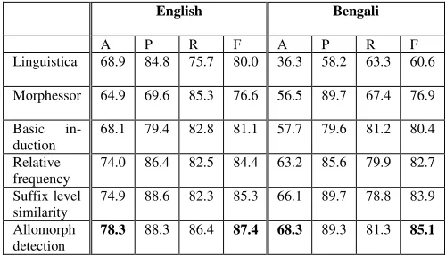
Results for English and BengaliThe baseline systems. We use two publicly
avail-able and widely used unsupervised morphological learning systems -- Goldsmith’s (2001) Linguis-tica11 and Creutz and Lagus’s (2005) Morphessor 1.012 -- as our baseline systems. The first two rows of Table 3 show the results of these systems for our test sets (with all the training parameters set to their default values). As we can see, Linguistica performs substantially better for English in terms of both exact accuracy and F-score, whereas Mor-phessor outperforms Linguistica for Bengali.
Our segmentation algorithm. Results of our
segmentation algorithm are shown in rows 3-6 of Table 3. Specifically, row 3 shows the results of our basic segmentation system as described in Sec-tion 3. Rows 4-6 show the results where our three techniques (i.e. relative frequency, suffix level
9 Words of length less than 4 do not have any morphological segmentation in
English. Hence, by imposing this length restriction on the words in our test set, we effectively make the evaluation more challenging. This is also the reason for our using words that are at least 3-character long in the Bengali test set.
10 See http://www.cis.hut.fi/morphochallenge2005/evaluation.shtml for details. 11 http://humanities.uchicago.edu/faculty/goldsmith/Linguistica2000/ 12 http://www.cis.hut.fi/projects/morpho/
similarity and allomorph detection) are incorpo-rated into the basic system one after the other. It is worth mentioning that (1) our basic algorithm al-ready outperforms the baseline systems in terms of both exact accuracy and F-score; and (2) while each of our additions to the basic algorithm boosts system performance, relative corpus frequency and allomorph detection contribute to performance im-provements particularly significantly. As we can see, the best segmentation performance is achieved when all of our three additions are applied to the basic algorithm.
English Bengali
A P R F A P R F
Linguistica 68.9 84.8 75.7 80.0 36.3 58.2 63.3 60.6
Morphessor 64.9 69.6 85.3 76.6 56.5 89.7 67.4 76.9
Basic
in-duction 68.1 79.4 82.8 81.1 57.7 79.6 81.2 80.4 Relative
frequency 74.0 86.4 82.5 84.4 63.2 85.6 79.9 82.7 Suffix level
similarity 74.9 88.6 82.3 85.3 66.1 89.7 78.8 83.9 Allomorph
[image:8.612.306.556.224.368.2]detection 78.3 88.3 86.4 87.4 68.3 89.3 81.3 85.1
Table 3: Results (reported in terms of exact accu-racy (A), precision (P), recall (R) and F-score (F))
8.3
PASCAL Challenge ResultsTo get an idea of how our algorithm performs in comparison to the PASCAL participants, we con-ducted evaluations on the PASCAL datasets for English, Finnish and Turkish. Table 4 shows the F-scores of four segmentation algorithms for these three datasets: the best-performing PASCAL sys-tem (Winner), Morphessor, our syssys-tem that uses the basic morpheme induction algorithm (Basic), and our system with all three extensions incorpo-rated (Complete). Below we discuss these results.
English. There are 533 test cases in this dataset.
Using the vocabulary created as described in Sec-tion 8.1, our Complete algorithm achieves an F-score of 79.4%, which outperforms the winner (Keshava and Pitler, 2006) by 2.6%. Although our basic morpheme induction algorithm is similar to that of Keshava and Pitler, a closer examination of the results reveals that F-score increases signifi-cantly with the incorporation of relative frequency and allomorph detection.
Finnish and Turkish. The real challenge in the
and Turkish due to their morphological richness. We use the 400K and 300K most frequent words from the Finnish and Turkish datasets provided by the organizers as our vocabulary. When tested on the gold standard of 661 Finnish and 775 Turkish words, our Complete system achieves F-scores of 65.2% and 66.2%, which are better than the win-ner’s scores (Bernhard (2006)). In addition, Com-plete outperforms Basic by 3-6% in F-score; these results suggest thatthe new techniques proposed in this paper (especially allomorph detection) are also very effective for Finnish and Turkish.
English Finnish Turkish
Winner 76.8 64.7 65.3
Morphessor 66.2 66.4 70.1
Basic 75.8 59.2 63.4
Complete 79.4 65.2 66.2
Table 4: F-scores for the PASCAL gold standards As mentioned in the introduction, none of the participating PASCAL systems offers robust per-formance across different languages. For instance, Keshava and Pitler’s algorithm, the winner for English, has F-scores of only 47% and 54% for Finnish and Turkish respectively, whereas Bern-hard’s algorithm, the winner for Finnish and Turk-ish, achieves an F-score of only 66% for English. On the other hand, our algorithm outperforms the winners for all the languages in the competition,
demonstrating its robustness across languages. Finally, although Morphessor achieves better re-sults for Turkish and Finnish than our Complete system, it performs poorly for English, having an F-score of only 66.2%. On the other hand, our re-sults for Finnish and Turkish are not significantly poorer than those of Morphessor.
9
Conclusions
We have presented an unsupervised word segmen-tation algorithm that offers robust performance across languages with different levels of morpho-logical complexity. Our algorithm not only outper-forms Linguistica and Morphessor for English and Bengali, but also compares favorably to the best-performing PASCAL morphological parsers when evaluated against all three target languages --English, Turkish, and Finnish -- in the Challenge. Experimental results indicate that the use of rela-tive corpus frequency for incorrect attachment de-tection and the induction of orthographic rules and
allomorphs have contributed to the performance of our algorithm particularly significantly.
References
R. H. Baayen, R. Piepenbrock and L. Gulikers. 1996. The CELEX2 lexical database (CD-ROM), LDC, Univ of Pennsylvania, Philadephia, PA.
D. Bernhard. 2006. Unsupervised morphological segmentation based on segment predictability and word segment align-ment. In PASCAL Challenge Workshop on Unsupervised Segmentation of Words into Morphemes.
M. R. Brent, S. K. Murthy and A. Lundberg. 1995. Discover-ing morphemic suffixes: A case study in minimum descrip-tion length inducdescrip-tion. In Proceedings of the Fifth International Workshop on AI and Statistics.
M. Creutz. 2003. Unsupervised segmentation of words using prior distributions of morph length and frequency. In Pro-ceedings of the ACL, pages 280-287.
M. Creutz and K. Lagus. 2005. Unsupervised morpheme seg-mentation and morphology induction from text corpora us-ing Morfessor 1.0. In Computer and Information Science, Report A81, Helsinki University of Technology.
S. Dasgupta and V. Ng. 2007. Unsupervised word segmenta-tion for Bangla. In Proceedings of ICON, pages 15-24. H. DéJean. 1998. Morphemes as necessary concepts for
struc-tures discovery from untagged corpora. In Workshop on Paradigms and Grounding in Natural Language Learning, pages 295-299.
D. Freitag. 2005. Morphology induction from term clusters. In Proceedings of CoNLL, pages 128-135.
J. Goldsmith. 2001. Unsupervised learning of the morphology of a natural language. In Computational Linguistics 27(2), pages 153-198.
Z. Harris. 1955. From phoneme to morpheme. In Language, 31(2): 190-222.
S. Keshava and E. Pitler. 2006. A simpler, intuitive approach to morpheme induction. In PASCAL Challenge Workshop on Unsupervised Segmentation of Words into Morphemes. K. Koskenniemi. 1983. Two-level morphology: a general
computational model for word-form recognition and pro-duction. Publication No. 11. Helsinki: University of Hel-sinki Department of General Linguistics.
P. Schone and D. Jurafsky. 2001. Knowledge-free induction of inflectional morphologies. In Proceedings of the NAACL, pages 183-191.
M. G. Snover and M. R. Brent. 2001. A Bayesian model for morpheme and paradigm identification. In Proceedings of the ACL, pages 482-490.