Proceedings of the First International Workshop on Language Cognition and Computational Models, pages 1–10 Santa Fe, New Mexico, United States, August 20, 2018.
1
A Compositional Bayesian Semantics for Natural Language
Jean-Philippe Bernardy Rasmus Blanck Stergios Chatzikyriakidis Shalom Lappin University of Gothenburg
Abstract
We propose a compositional Bayesian semantics that interprets declarative sentences in a natu-ral language by assigning them probability conditions. These are conditional probabilities that estimate the likelihood that a competent speaker would endorse an assertion, given certain hy-potheses. Our semantics is implemented in a functional programming language. It estimates the marginal probability of a sentence through Markov Chain Monte Carlo (MCMC) sampling of objects in vector space models satisfying specified hypotheses. We apply our semantics to ex-amples with several predicates and generalised quantifiers, including higher-order quantifiers. It captures the vagueness of predication (both gradable and non-gradable), without positing a pre-cise boundary for classifier application. We present a basic account of semantic learning based on our semantic system. We compare our proposal to other current theories of probabilistic semantics, and we show that it offers several important advantages over these accounts.
1 Introduction
In classical model theoretic semantics (Montague 1974; Dowty, Wall, and Peters 1981; Barwise and Cooper 1981) the interpretation of a declarative sentence is given as a set of truth conditions with Boolean values. This excludes vagueness from semantic interpretation, and it does not provide a natural frame-work for explaining semantic learning. Indeed, semantic learning involves the acquisition of classifiers (predicates), which seems to require probabilistic learning.1
Recently several theories of probabilistic semantics for natural language have been proposed to accom-modate both phenomena (van Eijck and Lappin 2012; Cooper et al. 2014; Cooper et al. 2015; Goodman and Lassiter 2015; Lassiter 2015; Lassiter and Goodman 2017; Sutton 2017). These accounts offer inter-esting ways of expressing vagueness, and suggestive approaches to semantic learning. They also suffer from a number of serious shortcomings, some of which we briefly discuss in Section 4.
In this paper we propose a compositional Bayesian semantics for natural language in which we assign probability rather than truth conditions to declarative sentences. We estimate the conditional probability of a sentence as the likelihood that an idealised competent speaker of the language would accept the assertion that the sentence expresses, given fixed interpretations of generalised quantifiers and certain other terms, and a set of specified hypotheses,pS(A|H). Sis a competent speaker of the language,A is the assertion that the sentence expresses, andHis the set of hypotheses on which we are conditioning the likelihood thatS will endorseA. On this approach assessing the probability of a sentence in the cir-cumstances defined by the hypotheses is an instance of evaluating the application of a classifier acquired through supervised learning, to a new argument (set of arguments).
Our semantics interprets sentences as probabilistic programs (Borgstr¨om et al. 2013). Section 2 gives a detailed description of our implementation. It involves encoding objects and properties as vectors in vector space models. Our system uses Markov Chain Monte Carlo (MCMC) sampling, as implemented
This work is licenced under a Creative Commons Attribution 4.0 International Licence. Licence details: http:// creativecommons.org/licenses/by/4.0/.
1See (Clark and Lappin 2011) for a discussion of computational learning and probabilistic learning models for natural
in WebPPL (Goodman and Stuhlm¨uller 2014), a lightweight version of Church (Goodman et al. 2008), and it estimates the marginal probabilities of predications and quantified sentences relative to the models satisfying the constraints of an asserted set of hypotheses (pS(A|H)).
We give examples of inferences involving several generalised quantifiers, including higher-order quan-tifiers (in the sense of Barwise and Cooper (1981)) likemost. Our semantics uses the same vector space models and sampling mechanism to express both the vagueness of gradable predicates, liketall, and of ordinary property terms, such asredandchair.
Our semantic framework does not require extensive lexically specified content or pragmatic knowledge statements to estimate the parameters of our vector space models. It also does not posit boundary values (hard coded or contextually specified) for the application of a predicate to an argument.
The system that we describe here is a prototype that offers a proof of concept for our approach. A robust, wide coverage version of this system will be useful for a variety of tasks. Three examples are as follows.
First, we intend to encode both semantic and real world knowledge as priors in our models. These will sustain probabilistic inferencing that will support text understanding and question answering in a way analogous to that in which Bayesian Networks are used for inference and knowledge representation in restricted domains. Second, we envisage an integration of visual and other non-linguistic vector representations into our models. This will facilitate the evaluation of candidate descriptions of images and scenes. It will also allow us to assess the relative accuracy of statements concerning these scenes. Finally, our system could be used as a filter on machine translation. Source and target sentences are expected to share the same probability values for the same models. The success which our framework achieves in these applications will provide criteria for evaluating it.
In Section 3 we present an outline of our implemented system for semantic learning, that extends our compositional semantics to the probabilistic acquisition of classifiers.
In Section 4 we compare our system to recent work in probabilistic semantics.
Finally, in Section 5 we state the main conclusions of our research, and we indicate the issues that we will address in future work.
2 An Implemented Probabilistic Semantics
Our semantics draws inspiration from (i) Montague semantics, (ii) vector space models, and (iii) Bayesian inference. Additionally, the implementation is guided by programming language theory. At the front-end we rely on a precise semantics for probabilistic programming, provided by Borgstr¨om et al., using their effect system to make explicit the sampling of parameters and observations. At the backend, we estimate probabilities using MCMC sampling, as described by Goodman et al. (2008). The imple-mentation is encoded as a Haskell library. It makes effects explicit using a monadic system, with calls into Goodman’s WebPPL language for probability approximation.2
Following Montague, our semantics assumes an assignment from syntactic categories to types. These assignments are given in Haskell as follows:
typePred =Ind →Prop typeMeasure=Ind →Scalar typeAP =Measure
typeCN =Ind →Prop typeVP =Ind →Prop typeNP =VP →Prop typeQuant =CN →NP
While Montague leaves individuals Ind as an abstract type, we give it a concrete definition. We represent individuals as vectors, and propositions as (probabilistic) Booleans. Additionally, adjectival phrases are treated as scalars, and so they are expressed by a real number.
2The code for our system is available at https://github.com/GU-CLASP/
Crucially, the evaluation of every expression is probabilistic. The meaning of each expression in our semantic domain is itself a probability distribution, whose value can be computed symbolically using the rules provided by Borgstr¨om et al. (2013), or approximated with a tool such as WebPPL.
2.1 Individuals and Predicates
We can illustrate these concepts by a simple example, written in Haskell syntax, using our front end.
modelSimplest =do p ←newPred x ←newInd return (p x)
The functionmodelSimplestdeclares a predicatepand an individualx, and probabilistically evaluates the proposition “xsatisfiesp”. Note that “newPred” and “newInd” have theeffectof sampling over their respective distribution (we clarify those shortly), and so have monadic types. In the absence of further information, an arbitrary predicate has an even chance to hold of an arbitrary individual. Running the model, using our implementation, gives the following approximate result:
false : 0.544 true : 0.456
The distribution of individuals is a multi-variate normal distribution of dimensionk, with a zero mean vector and a unit covariance matrix, and wherek is a hyperparameter of the system.
newInd =newVector
newVector =mapM (uncurry sampleGaussian) (replicate k (0,1))
Predicates are parameterised by a bias band a vector d, given by normalizing a vector sampled in the same multi-variate normal as individuals. Any individual x is said to satisfy the predicate if the expressionb+d·x >0is true. In code:
newMeasure =do
b←sampleGaussian 0 1 d ←newNormedVector return (λx →b+d ·x)
newPred =do m ←newMeasure return (λx →m x>0)
In addition to sampling random predicates and individuals, and evaluating expressions, we can make assumptions about them. We do this using theobserveprimitive of Borgstr¨om et al. (2013). The name of this primitive suggests that the agent observes a situation where a given proposition holds. In terms of MCMC sampling, if the argument to anobserve call is false, then the previously sampled parameters are discarded, and a fresh run of the program is performed. In fact, in the WebPPL implementation that we use, only a portion of the sampling history may be discarded (see (Goodman and Stuhlm¨uller 2014) for details.) A trivial model usingobserve is the following, where one evaluates the probability of an observed fact:
modelSimple=do p ←newPred x ←newInd observe (p x) return (p x)
Even when using our approximating implementation, evaluating the above model yields certainty.
2.2 Comparatives
We support scalar predicates and comparatives. The expressionb+d·xcan be interpreted as a degree to which the individualxsatisfies the property characterised by(b, d). Thus satisfying a scalar predicate is defined as follows:
is::Measure →Pred is m x =m x>0
And comparatives can be defined by comparing such measures:
more::Measure→Ind →Ind →Prop more m x y =m x>m y
Using these concepts we can define models like the following:
modelTall::P Scalar modelTall =do
tall ←newMeasure john ←newInd mary ←newInd
observe (more tall john mary)
return (is tall john)
That is, if we observe that “John is taller than Mary”, we will infer that “John is tall” is slightly more probable than “John is not tall”.
The exact probability values that the model produces will be influenced by the priors that we apply (such as the standard deviation of Gaussian distributions), in addition to the observations that we record. Further, MCMC sampling is an approximation method, thus the results will vary from run to run. In the rest of the paper we will show results obtained from a typical run. For the above example, we get:
true : 0.552 false : 0.448
2.3 Vague predicates
We support vague predication, by adding an uncertainty to each measure we make for the predicate in question. This is implemented through a Gaussian error with a given std. dev.σfor each measure.
vagueσ m x =m x +gaussian 0σ
modelTall::P Prop modelTall =do
tall ←vague 3<$>newMeasure john ←newInd
mary ←newInd
hyp (more tall john mary)
return (is tall john)
In this situation the tallness of John is more uncertain than before:
false : 0.512 true : 0.488
Additionally, a vague predicate allows apparently contradictory statements to hold, although with low probability, giving a fuzzy quality to the system. For example:
modelTallContr::P Prop modelTallContr =do
john ←newInd mary ←newInd
return (more tall john mary ∧more tall mary john)
false : 0.77 true : 0.23
2.4 Generalised Universal Quantifiers
We now turn to generalised quantifiers. We need to interpret sentences such as “most birds fly” compo-sitionally. On a standard reading, “most” can be seen as a constraint on a ratio between the cardinality of sets.
most(cn, vp) = #{x:cn(x)∧vp(x)}
#{x:cn(x)} > θ. (1)
for a suitable thresholdθ. Translated into a probabilistic framework, we posit that the expected value of vp(x)given thatcn(x)holds should be greater thanθ.
most(cn, vp) =E(1(vp(x))|cn(x))> θ (2)
where1is an indicator function, such that1(true) = 1and1(f alse) = 0.In general,cnandvpmay depend on probabilistic variables, and thus the above equation isitself probabilistic.
While taking the expected value is not an operation found in the language presented by Borgstr¨om et al. (2013), it is not difficult to extend their framework in this direction, because the expected value can be given a definite symbolic form:
most(cn, vp) =
R
IndfN(x)1(cn(x)∧vp(x))dx
R
IndfN(x)1(cn(x))dx
> θ (3)
wherefN denotes the density of the multivariate gaussian distribution for individuals. Further, the above can be implemented in many probabilistic programming languages, including WebPPL. In Haskell code, we write:
most::Quant
most cn vp =expectedIndicator p> θ
wherep =dox ←newInd observe(cn x)
return(vp x)
That is, we create a probabilistic program p, which samples over all individualsx which satisfycn, and we evaluatevp(x). The compound statement is satisfied if the expected value of the program p, itself evaluated using an inner MCMC sampling procedure, is larger than θ. In our examples, we let θ= 0.7. Other generalised quantifiers can be defined in the same way with a different value forθ— in our examples we definemanywithθ= 0.6.3
On this basis, we make inferences of the following kind. “If many chairs have four legs, then it is likely that any given chair has four legs”. We model this sentence as follows:
chairExample1 =do chair ←newPred fourlegs ←newPred
observe (many chair fourlegs) x ←newIndSuch [chair] return (fourlegs x)
3It is possible, in fact desirable, to letθbe sampled (say from a beta distribution) so that its posterior would depend on
true : 0.821 false : 0.179
The model samples all possible parameter values (vectors/biases) for chairs and four-legged objects. Then, it discards all parameters such thatE(1(f our−legged(y))|chair(y))≤θfor a random individ-ualy. In the implementation this expected value is approximated by first doing an independent sampling of a number of individualsysuch thatchair(y)holds, and then checking the value off our−legged(y)
for this sample.
The evaluation of the last two statements, corresponding toE(f our−legged(x))|chair(x), is done using another sampling of individuals, but retaining the values for chair and four-legged parameters identified in the previous sampling.
Interestingly, because the models that we are building implement generalized quantifiers through cor-relation of predicates, we get ‘inverse’ corcor-relation as well. Therefore, assuming that “many chairs have four legs”, and in the absence of further information, and given an individualxwith four legs, we will predict a high probability forchair(x).
chairExample2 ::P Prop chairExample2 =do
chair ←newPred fourlegs ←newPred
observe (many chair fourlegs) x ←newIndSuch [fourlegs] return (chair x)
true : 0.653 false : 0.347
The model’s assumptions can be augmented with the hypothesis that most individuals are not chairs. This will lower the probability of being a chair appropriately.
chairExample3 ::P Prop chairExample3 =do
chair ←newPred fourlegs ←newPred
observe (many chair fourlegs)
observe (most anything (not0◦chair)) x ←newIndSuch [fourlegs]
return (chair x)
false : 0.779 true : 0.221
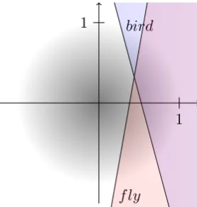
We conclude this section with a more complex example inference involving three predicates and four propositions. Assume that
1. Most animals do not fly.
2. Most birds fly.
3. Every bird is an animal.
Can we conclude that “most animals are not birds”? We model the example as follows:
birdExample =do animal ←newPred bird ←newPred fly ←newPred
observe (every bird animal) return (most animal (not0◦bird))
And it concludes with overwhelming probability:
true : 0.941 false : 0.059
This result can be explained by the fact that only models similar to the one pictured in Figure 1 conform to the assumptions. One way to satisfy “every bird is an animal” is to assume that “animal” holds for every individual, because this is compatible with all hypotheses. Then “most animals don’t fly” implies that the “fly” predicate has a large (negative) bias. Finally, “most birds fly” can be satisfied only if “fly” is highly correlated with “bird” (the predicate vectors have similar angles),and if the bias of “bird” is even more negative than that of “fly”. Consequently, “bird” also has a large negative bias, and the conclusion holds.
3 Semantic Learning
Bayesian models can adapt to new observations, giving rise to learning. We have seen that our frame-work takes account of data provided in the form of qualitative statements, including those made with generalised quantifiers. We can also accommodate information in a sequence of observed situations.
Consider the following data (which we have taken fromhttps://en.wikipedia.org/wiki/ Naive_Bayes_classifier).
Person height (feet) weight (lbs) foot size(inches)
male 6 180 12
male 5.92 190 11
male 5.58 170 12
male 5.92 165 10
female 5 100 6
female 5.5 150 8
female 5.42 130 7
female 5.75 150 9
We feed the person and weight data into our system to see if it can learn a correlation between these two random variables.
model::P Prop model =do
weight ←newMeasure
bird
f ly
[image:7.595.229.368.523.669.2]1 1
isMale ←newPred
letsampleWith::Bool →Float →P Ind sampleWith male w =do
s ←newInd
observe (isMale s‘iff‘constant male) observeEqual (weight s) (constant w) return s
←sampleWith True 1.80
←sampleWith True 1.90
←sampleWith True 1.70
←sampleWith True 1.65
←sampleWith False1.00
←sampleWith False1.50
←sampleWith False1.30
←sampleWith False1.50
x ←newInd
observeEqual (weight x) 1.9 return (isMale x)
The data is provided as a series of observations. The Boolean observations use the usual observe
primitive. To handle continuous data, we must add a new primitive in our implementation. In principle we could add a hard constraint on the measure of any scalar predicate, and the posterior would simply select points which satisfy exactly this constraint. However, because we are using MCMC sampling, this strategy would discard all samples that do not satisfy the constraint exactly. But because precise satisfaction of a constraint is stochastically impossible, all samples would be discarded and we would never obtain an approximation for the posteriors.
To avoid this problem we retain samples which do not satisfy the equality exactly, but with a specified probability, given by the expression e−d2, wheredis the distance between the predicted and observed values.
With this implementation our model predicts that an individual of weight1.9is male with the following probabilities.
true : 0.57805 false : 0.42195
A more direct way to identify the learned correlation between weight and maleness is by measuring the cosine of the angle between the weight and male vectors. The posterior adheres to the following distribution, which indicates a strong correlation.
-0.5 0 0.5 1 1.5 2 2.5 3 3.5 4 4.5 5
-1.5 -1 -0.5 0 0.5 1 1.5
4 Related Work
true. This proposal is not implemented, and it is unclear how the worlds to which probability is assigned can be represented in a computationally tractable way.4 Van Eijck and Lappin also suggest an account of semantic learning. It seems to require the wholistic acquisition of all the classifier predicates in a language in a correlated way.
Our system avoids these problems. Our models sample only the individuals and properties (vector dimensions) required to estimate the probability of a given set of statements. Learning is achieved for restricted sets of predicates with these models.
Cooper et al. (2014) and Cooper et al. (2015) develop a compositional semantics within a probabilistic type theory (ProbTTR). On their approach the probability of a sentence is a judgment on the likelihood that a given situation is of a particular type, specified in terms of ProbTTR. They also sketch a Bayesian treatment of semantic learning.
Cooper et al.’s semantics is not implemented, and so it is not entirely clear how probabilities for sen-tences are computed in their system. They do not offer an explicit treatment of vagueness or probabilistic inference. It is also not obvious that their type theory is relevant to a viable compositional probabilistic semantics.
Sutton (2017) uses a Bayesian view of probability to support a resolution of classical philosophical problems of vagueness in degree predication. His treatment of these problems is insightful, and it seems to be generally compatible with our implemented semantics. But it operates at a philosophical level of abstraction, and so a clear comparison is not possible.
Goodman and Lassiter (2015) and Lassiter and Goodman (2017) construct a probabilistic semantics implemented in WebPPL. They construe the probability of a declarative sentence as the most highly valued interpretation that a hearer assigns to the utterance of a speaker in a specified context. The Goodman–Lassiter account requires the specification of considerable amounts of real world knowledge and lexical information in order to support pragmatic inference. It appears to require the existence of a univocal, non-vague speaker’s meaning that hearers seek to identify by distributing probability among alternative readings. Goodman and Lassiter posit a boundary cut off point parameter for graded modi-fiers, where the value of this parameter is determined in context. They adopt a classical Montagovian treatment of generalised quantifiers. They also do not offer a theory of semantic learning.
By contrast we take the probability value of a sentence as the likelihood that a competent speaker would endorse an assertion given certain assumptions (hypotheses). Therefore, predication remains in-trinsically vague. We do not assume the existence of a sharply delimited non-probabilistic reading for a predication that hearers attempt to converge on through estimating the probability of alternative read-ings. All predication consists in applying a classifier to new instances on the basis of supervised training. We do not posit a contextually dependent cut off boundary for graded predicates, but we suggest an integrated approach to graded and non-graded predication on which both types of property term allow for vague borders. Further advantages of our account include a probabilistic treatment of generalised quantifiers, which includes higher-order quantifiers likemost, and a basic theory of semantic learning that is a straightforward extension of our sampling procedures for computing the marginal probability of a sentence in a model.
5 Conclusions and Future Work
We have presented a compositional Bayesian semantics for natural language, implemented in the func-tional programming language WebPPL. We represent objects and properties as vectors inn-dimensional vector spaces. Our system computes the marginal probability of a declarative sentence through MCMC sampling in Bayesian models constrained by specified hypotheses.
Our semantic framework provides straightforward treatments of vagueness in predication, gradable predicates, comparatives, generalised quantifiers, and probabilistic inferences across several property dimensions with generalised quantifiers. It avoids some of the limitations of other current probabilistic semantic theories.
In future work we will extend the syntactic and semantic coverage of our framework. We will improve our modelling and sampling mechanisms to accommodate large scale applications more efficiently and robustly. Finally, we will develop our Bayesian learning theory to handle more complex cases of classifier acquisition.
Acknowledgements
The research reported in this paper was supported by grant 2014-39 from the Swedish Research Council, which funds the Centre for Linguistic Theory and Studies in Probability (CLASP) in the Department of Philosophy, Linguistics, and Theory of Science at the University of Gothenburg. We are grateful to our colleagues in CLASP for helpful discussion of many of the ideas presented here.
References
Barwise, J. and R. Cooper (1981). “Generalised Quantifiers and Natural Language”. In:Linguistics and Philosophy4, pp. 159–219.
Borgstr¨om, Johannes et al. (2013). “Measure Transformer Semantics for Bayesian Machine Learning”. In:Logical Methods in Computer Science9, pp. 1–39.
Clark, A. and S. Lappin (2011).Linguistic Nativism and the Poverty of the Stimulus. Chichester, West Sussex, and Malden, MA: Wiley-Blackwell.
Cooper, R. et al. (2014). “A Probabilistic Rich Type Theory for Semantic Interpretation”. In:Proceedings of the EACL 2014 Workshop on Type Theory and Natural Language Semantics (TTNLS). Gothenburg, Sweden: Association of Computational Linguistics, pp. 72–79.
– (2015). “Probabilistic Type Theory and Natural Language Semantics”. In:Linguistic Issues in Lan-guage Technology10, pp. 1–43.
Dowty, D. R., R. E. Wall, and S. Peters (1981). Introduction to Montague Semantics. Dordrecht: D. Reidel.
Goodman, N. and D. Lassiter (2015). “Probabilistic Semantics and Pragmatics: Uncertainty in Language and Thought”. In:The Handbook of Contemporary Semantic Theory, Second Edition. Ed. by S. Lappin and C. Fox. Malden, Oxford: Wiley-Blackwell, pp. 143–167.
Goodman, N. et al. (2008). “Church: a Language for Generative Models”. In:Proceedings of the 24th Conference Uncertainty in Artificial Intelligence (UAI), pp. 220–229.
Goodman, Noah D and Andreas Stuhlm¨uller (2014).The Design and Implementation of Probabilistic Programming Languages.http://dippl.org. Accessed: 2018-4-17.
Lappin, Shalom (2015). “Curry Typing, Polymorphism, and Fine-Grained Intensionality”. In:The Hand-book of Contemporary Semantic Theory, Second Edition. Ed. by Shalom Lappin and Chris Fox. Malden, MA and Oxford: Wiley-Blackwell, pp. 408–428.
Lassiter, D. (2015). “Adjectival modification and gradation”. In:The Handbook of Contemporary Seman-tic Theory, Second Edition. Ed. by S. Lappin and C. Fox. Malden, Oxford: Wiley-Blackwell, pp. 655– 686.
Lassiter, Daniel and Noah Goodman (2017). “Adjectival Vagueness in a Bayesian Model of Interpreta-tion”. In:Synthese194, pp. 3801–3836.
Montague, Richard (1974). “The Proper Treatment of Quantification in Ordinary English”. In:Formal Philosophy. Ed. by Richmond Thomason. New Haven: Yale UP.
Sutton, Peter R. (2017). “Probabilistic Approaches to Vagueness and Semantic Competency”. In: Erken-ntnis.