TwiSE at SemEval-2016 Task 4: Twitter Sentiment Classification
Georgios Balikas and Massih-Reza Amini
University of Grenoble-Alpes
Abstract
This paper describes the participation of the team “TwiSE” in the SemEval 2016 challenge. Specifically, we participated in Task 4, namely “Sentiment Analysis in Twitter” for which we implemented sentiment classification systems for subtasks A, B, C and D. Our approach consists of two steps. In the first step, we generate and validate diverse feature sets for twitter sentiment evaluation, inspired by the work of participants of previous editions of such challenges. In the second step, we focus on the optimization of the evaluation measures of the different subtasks. To this end, we examine different learning strategies by validating them on the data provided by the task organisers. For our final submissions we used an ensemble learning approach (stacked generalization) for Subtask A and single linear models for the rest of the subtasks. In the official leaderboard we were ranked 9/35, 8/19, 1/11 and 2/14 for subtasks A, B, C and D respectively. The code can be found at https://github.com/ balikasg/SemEval2016-Twitter_ Sentiment_Evaluation.
1 Introduction
During the last decade, short-text communication forms, such as Twitter microblogging, have been widely adopted and have become ubiquitous. Us-ing such forms of communication, users share a va-riety of information. However, information concern-ing one’s sentiment on the world around her has at-tracted a lot of research interest (Nakov et al., 2016; Rosenthal et al., 2015).
Working with such short, informal text spans poses a number of different challenges to the Natu-ral Language Processing (NLP) and Machine Learn-ing (ML) communities. Those challenges arise from the vocabulary used (slang, abbreviations, emojis) (Maas et al., 2011), the short size, and the complex linguistic phenomena such as sarcasm (Rajadesin-gan et al., 2015) that often occur.
We present, here, our participation in Task 4 of SemEval 2016 (Nakov et al., 2016), namely Senti-ment Analysis in Twitter. Task 4 comprised five dif-ferent subtasks: Subtask A: Message Polarity Clas-sification, Subtask B: Tweet classification according to a two-point scale, Subtask C: Tweet classification according to a five-point scale, Subtask D: Tweet quantification according to a two-point scale, and Subtask E: Tweet quantification according to a five-point scale. We participated in the first four subtasks under the team name “TwiSE” (Twitter Sentiment Evaluation). Our work consists of two steps: the preprocessing and feature extraction step, where we implemented and tested different feature sets pro-posed by participants of the previous editions of Se-mEval challenges (Tang et al., 2014; Kiritchenko et al., 2014a), and the learning step, where we inves-tigated and optimized the performance of different learning strategies for the SemEval subtasks. For Subtask A we submitted the output of a stacked gen-eralization (Wolpert, 1992) ensemble learning ap-proach using the probabilistic outputs of a set of lin-ear models as base models, whereas for the rest of the subtasks we submitted the outputs of single mod-els, such as Support Vector Machines and Logistic
Regression.1
The remainder of the paper is organised as fol-lows: in Section 2 we describe the feature extraction and the feature transformations we used, in Section 3 we present the learning strategies we employed, in Section 4 we present a part of the in-house val-idation we performed to assess the models’ perfor-mance, and finally, we conclude in Section 5 with remarks on our future work.
2 Feature Engineering
We present the details of the feature extraction and transformation mechanisms we used. Our approach is based on the traditional N-gram extraction and on the use of sentiment lexicons describing the sen-timent polarity of unigrams and/or bigrams. For the data pre-processing, cleaning and tokenization2
as well as for most of the learning steps, we used Python’s Scikit-Learn (Pedregosa et al., 2011) and NLTK (Bird et al., 2009).
2.1 Feature Extraction
Similar to (Kiritchenko et al., 2014b) we extracted features based on the lexical content of each tweet and we also used sentiment-specific lexicons. The features extracted for each tweet include:
• N-grams with N ∈ [1,4], character grams of dimensionM ∈[3,5],
• # of exclamation marks, # of question marks, # of both exclamation and question marks,
• # of capitalized words and # of elongated words,
• # of negated contexts; negation also affected
theN-grams features by transforming a word win a negated context tow N EG,
• # of positive emoticons, # of negative
cons and a binary feature indicating if emoti-cons exist in a given tweet, and
1To enable replicability we make the code we used available at https://github.com/balikasg/ SemEval2016-Twitter_Sentiment_Evaluation.
2We adapted the tokenizer provided at http:// sentiment.christopherpotts.net/tokenizing. html
• Part-of-speech (POS) tags (Gimpel et al., 2011) and their occurrences partitioned regarding the positive and negative contexts.
With regard to the sentiment lexicons, we used:
• manual sentiment lexicons: the Bing liu’s lexi-con (Hu and Liu, 2004), the NRC emotion lex-icon (Mohammad and Turney, 2010), and the MPQA lexicon (Wilson et al., 2005),
• # of words in positive and negative context be-longing to the word clusters provided by the CMU Twitter NLP tool3
• positional sentiment lexicons: sentiment 140
lexicon (Go et al., 2009) and the Hashtag Sen-timent Lexicon (Kiritchenko et al., 2014b)
We make, here, more explixit the way we used the sentiment lexicons, using the Bing Liu’s lexicon as an example. We treated the rest of the lexicons sim-ilarly. For each tweet, using the Bing Liu’s lexi-con we obtain a 104-dimensional vector. After to-kenizing the tweet, we count how many words (i) in positive/negative contenxts belong to the posi-tive/negative lexicons (4 features) and we repeat the process for the hashtags (4 features). To this point we have 8 features. We generate those 8 features for the lowercase words and the uppercase words. Finally, for each of the 24 POS tags the (Gimpel et al., 2011) tagger generates, we count how many words in positive/negative contenxts belong to the positive/negative lexicon. As a results, this gener-ates2×8 + 24×4 = 104features in total for each
tweet.
For each tweet we also used the distributed repre-sentations provided by (Tang et al., 2014) using the min, max and average composition functions on the vector representations of the words of each tweet.
2.2 Feature Representation and Transformation
We describe the different representations of the ex-tractedN-grams and character-grams we compared when optimizing our performance on each of the classification subtasks we participated. In the rest of this subsection we refer to both N-grams and
character-grams as words, in the general sense of letter strings. We evaluated two ways of represent-ing such features: (i) a bag-of-words representation, that is for each tweet a sparse vector of dimension
|V| is generated, where |V| is the vocabulary size, and (ii) a hashing function, that is a fast and space-efficient way of vectorizing features, i.e. turning ar-bitrary features into indices in a vector (Weinberger et al., 2009). We found that the performance using hashing representations was better. Hence, we opted for such representations and we tuned the size of the feature space for each subtask.
Concerning the transformation of the features of words, we compared the tf-idf weighing scheme and the α-power transformation. The latter,
trans-forms each vector x = (x1, x2, . . . , xd) to x0 =
(xα1, xα2, . . . , xαd)(Jegou et al., 2012). The main
in-tuition behind theα-power transformation is that it
reduces the effect of the most common words. Note that this is also the rationale behind theidf weight-ing scheme. However, we obtained better results us-ing theα-power transformation. Hence, we tunedα
separately for each of the subtasks.
3 The Learning Step
Having the features extracted we experimented with several families of classifiers such as linear models, maximum-margin models, nearest neighbours ap-proaches and trees. We evaluated their performance using the data provided by the organisers, which were already split in training, validation and testing parts. Table 1 shows information about the tweets we managed to download. From the early valida-tion schemes, we found that the two most competi-tive models were Logistic Regression from the fam-ily of linear models, and Support Vector Machines (SVMs) from the family of maximum margin mod-els. It is to be noted that this is in line with the previ-ous research (Mohammad et al., 2013; B¨uchner and Stein, 2015).
3.1 Subtask A
Subtask A concerns a multiclass classification prob-lem, where the general polarity of tweets has to be classified in one among three classes: “Positive”, “Negative” and “Neutral”, each denoting the tweet’s overall polarity. The evaluation measure used for the
subtask is the Macro-F1 measure, calculated only
for the Positive and Negative classes (Nakov et al., 2016).
Inspired by the wining system of SemEval 2015 Task 10 (B¨uchner and Stein, 2015) we decided to employ an ensemble learning approach. Hence, our goal is twofold: (i) to generate a set of models that perform well as individual models, and (ii) to select a subset of models of (i) that generate diverse out-puts and to combine them using an ensemble learn-ing step that would result in lower generalization er-ror.
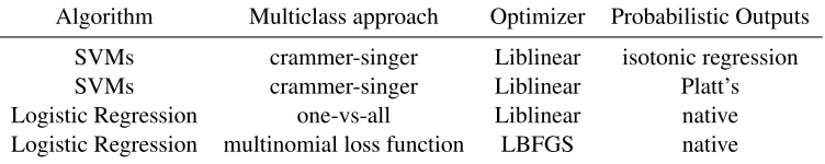
We trained four such models as base models. Their details are presented in Table 2. In the stacked generalization approach we employed, we found that by training the second level classifier on the probabilistic outputs, instead of the predictions of the base models, yields better results. Logistic Re-gression generates probabilities as its outputs. In the case of SVMs, we transformed the confidence scores into probabilities using two methods, after adapting them to the multiclass setting: the Platt’s method (Platt and others, 1999) and the isotonic regression (Zadrozny and Elkan, 2002). To solve the opti-mization problems of SVMs we used the Liblinear solvers (Fan et al., 2008). For Logistic Regression we used either Liblinear or LBFGS, with the latter being a limited memory quasi Newton method for general unconstrained optimization problems (Yu et al., 2011). To attack the multiclass problem, we se-lected among the traditional one-vs-rest approach, the crammer-singer approach for SVMs (Crammer and Singer, 2002), or the multinomial approach for Logistic Regression (also known as MaxEnt classi-fier), where the multinomial loss is minimised across the entire probability distribution (Malouf, 2002).
integrat-Train Development DevTest Test Subtask A 5,500 1,831 1,791 32,009 Subtask B & D 4,346 1,325 1,417 10,551 Subtask C & E 5,482 1,810 1,778 20,632
Table 1:Size of the data used for training and development purposes. We only relied on the SemEval 2016 datasets.
Algorithm Multiclass approach Optimizer Probabilistic Outputs SVMs crammer-singer Liblinear isotonic regression SVMs crammer-singer Liblinear Platt’s Logistic Regression one-vs-all Liblinear native Logistic Regression multinomial loss function LBFGS native
Table 2:Description of the base learners used in the stacked generalization approach.
ing it in the stacked generalization.
Having the fine-tuned probability estimates for each of the instances of the test sets and for each of the base learners, we trained a second layer clas-sifier using those fine-grained outputs. For this, we used SVMs, using the crammer-singer approach for the multi-class problem, which yielded the best per-formance in our validation schemes. Also, since the classification problem is unbalanced in the sense that the three classes are not equally represented in the training data, we assigned weights to make the prob-lem balanced. Those weights were inversely propor-tional to the class frequencies in the input data for each class.
3.2 Subtask B
Subtask B is a binary classification problem where given a tweet known to be about a given topic, one has to classify whether the tweet conveys a posi-tive or a negaposi-tive sentiment towards the topic. The evaluation measure proposed by the organisers for this subtask is macro-averaged recall (MaR) over the positive and negative class.
Our participation is based on a single model. We used SVMs with a linear kernel and the Liblinear optimizer. We used the full feature set described in Section 2, after excluding the distributed embed-dings because in our local validation experiments we found that they actually hurt the performance. Sim-ilarly to subtask A and due to the unbalanced nature of the problem, we use weights for the classes of the problem. Note that we do not consider the topic of the tweet and we classify the tweet’s overall polarity.
Hence, we ignore the case where the tweet consists of more than one parts, each expressing different po-larities about different parts.
3.3 Subtask C
Subtask C concerns an ordinal classification prob-lem. In the framework of this subtask, given a tweet known to be about a given topic, one has to esti-mate the sentiment conveyed by the tweet towards the topic on a five-point scale. Ordinal classifica-tion differs from standard multiclass classificaclassifica-tion in that the classes are ordered and the error takes into account this ordering so that not all mistakes weigh equally. In the tweet classification problem for in-stance, a classifier that would assign the class “1” to an instance belonging to class “2” will be less pe-nalized compared to a classifier that will assign “-1” as the class . To this direction, the evaluation mea-sure proposed by the organisers is the macroaver-aged mean absolute error.
Similarly to Subtask B, we submitted the results of a single model and we classified the tweets ac-cording to their overall polarity ignoring the given topics. Instead of using one of the ordinal classifica-tion methods proposed in the bibliography, we use a standard multiclass approach. For that we use a Logistic Regression that minimizes the multinomial loss across the classes. Again, we use weights to cope with the unbalanced nature of our data. The distributed embeddings are excluded by the feature sets.
of an ordinal one. We evaluated a selection of methods described in (Pedregosa-Izquierdo, 2015) and in (Guti´errez et al., 2015). In both cases, the results achieved with the multiclass methods were marginally better and for simplicity we opted for the multiclass methods. We believe that this is due to the nature of the problem: the feature sets and es-pecially the fine-grained sentiment lexicons manage to encode the sentiment direction efficiently. Hence, assigning a class of completely opposite sentiment can only happen due to a complex linguistic phe-nomenon such as sarcasm. In the latter case, both methods may fail equally.
3.4 Subtask D
Subtask D is a binary quantification problem. In par-ticular, given a set of tweets known to be about a given topic, one has to estimate the distribution of the tweets across the Positive and Negative classes. For instance, having 100 tweets about the new iPhone, one must estimate the fractions of the Pos-itive and Negative tweets respectively. The organ-isers proposed a smoothed version of the Kullback-Leibler Divergence (KLD) as the subtask’s evalua-tion measure.
We apply a classify and count approach for this task (Bella et al., 2010; Forman, 2008), that is we first classify each of the tweets and we then count the instances that belong to each class. To this end, we compare two approaches both trained on the features sets of Section 2 excluding the distributed represen-tations: the standard multiclass SVM and a structure learning SVM that directly optimizes KLD (Esuli and Sebastiani, 2015). Again, our final submission uses the standard SVM with weights to cope with the imbalance problem as the model to classify the tweets. That is because the method of (Gao and Sebastiani, 2015) although competitive was outper-formed in most of our local validation schemes.
4 The evaluation framework
Before reporting the scores we obtained, we elabo-rate on our validation stelabo-rategy and the steps we used when tuning our models. in each of the subtasks we only used the data that were realised for the 2016 edition of the challenge. Our validation had the fol-lowing steps:
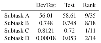
[image:5.612.336.514.68.144.2]DevTest Test Rank Subtask A 56.01 58.61 9/35 Subtask B 0.748 0.748 8/18 Subtask C 0.8121 0.72 1/11 Subtask D 0.00018 0.053 2/14
Table 3: The performance obtained on the “devtest” data and the SemEval 2016 Task 4 test data.
1. Training using the released training data,
2. validation on the validation data,
3. validation again, in the union of the devtest and trial data (when applicable), after retraining on training and validation data.
For each parameter, we selected its value by averag-ing the optimal parameters with respect to the out-put of the above-listed steps (2) and (3). It is to be noted, that we strictly relied on the data released as part of the 2016 edition of SemEval; we didn’t use past data.
We now present the performance we achieved both in our local evaluation schemas and in the offi-cial results released by the challenge organisers. Ta-ble 3 presents the results we obtained in the “De-vTest” part of the challenge dataset and the scores on the test data as they were released by the organ-isers. In the latter, we were ranked 9/35, 8/19, 1/11 and 2/14 for subtasks A, B, C and D respectively. Observe, that for subtasks A and B, using just the “devtest” part of the data as validation mechanism results in a quite accurate performance estimation.
5 Future Work
That was our first contact with the task of sentiment analysis and we achieved satisfactory results. We relied on features proposed in the framework of pre-vious SemEval challenges and we investigated the performance of different classification algorithms.
same line, we plan to improve our mechanism for handling negation. We have used a simple mech-anism where a negative context is defined as the group of words after a negative word until a punctu-ation symbol. However, our error analysis revealed that punctuation is rarely used in tweets. Finally, we plan to investigate ways to integrate more data in our approaches, since we only used this edition’s data.
The application of an ensemble learning ap-proach, is a promising direction towards the short text sentiment evaluation. To this direction, we hope that an extensive error analysis process will help us identify better classification systems that when inte-grated in our ensemble (of subtask A) will reduce the generalization error.
Acknowledgments
We would like to thank the organisers of the Task 4 of SemEval 2016, for providing the data, the guide-lines and the infrastructure. We would also like to thank the anonymous reviewers for their insightful comments.
References
[Bella et al.2010] Antonio Bella, Cesar Ferri, Jos´e Hern´andez-Orallo, and Maria Jose Ramirez-Quintana. 2010. Quantification via probability estimators. In
Data Mining (ICDM), 2010 IEEE 10th International Conference on, pages 737–742. IEEE.
[Bird et al.2009] Steven Bird, Ewan Klein, and Edward Loper. 2009. Natural Language Processing with Python. O’Reilly Media.
[B¨uchner and Stein2015] Matthias Hagen Martin Pot-thast Michel B¨uchner and Benno Stein. 2015. We-bis: An ensemble for twitter sentiment detection.
SemEval-2015, page 582.
[Crammer and Singer2002] Koby Crammer and Yoram Singer. 2002. On the algorithmic implementation of multiclass kernel-based vector machines.The Journal of Machine Learning Research, 2:265–292.
[Esuli and Sebastiani2015] Andrea Esuli and Fabrizio Se-bastiani. 2015. Optimizing text quantifiers for multi-variate loss functions. ACM Transactions on Knowl-edge Discovery from Data (TKDD), 9(4):27.
[Fan et al.2008] Rong-En Fan, Kai-Wei Chang, Cho-Jui Hsieh, Xiang-Rui Wang, and Chih-Jen Lin. 2008. Li-blinear: A library for large linear classification. The Journal of Machine Learning Research, 9:1871–1874. [Forman2008] George Forman. 2008. Quantifying counts and costs via classification. Data Mining and Knowledge Discovery, 17(2):164–206.
[Gao and Sebastiani2015] Wei Gao and Fabrizio Sebas-tiani. 2015. Tweet sentiment: From classifica-tion to quantificaclassifica-tion. In Proceedings of the 2015 IEEE/ACM International Conference on Advances in Social Networks Analysis and Mining 2015, pages 97– 104. ACM.
[Gimpel et al.2011] Kevin Gimpel, Nathan Schneider, Brendan O’Connor, Dipanjan Das, Daniel Mills, Jacob Eisenstein, Michael Heilman, Dani Yogatama, Jeffrey Flanigan, and Noah A Smith. 2011. Part-of-speech tagging for twitter: Annotation, features, and exper-iments. InProceedings of the 49th Annual Meeting of the Association for Computational Linguistics: Hu-man Language Technologies: short papers-Volume 2, pages 42–47. Association for Computational Linguis-tics.
[Go et al.2009] Alec Go, Richa Bhayani, and Lei Huang. 2009. Twitter sentiment classification using distant su-pervision.CS224N Project Report, Stanford, 1:12. [Guti´errez et al.2015] P.A. Guti´errez, M. P´erez-Ortiz,
J. S´anchez-Monedero, F. Fernandez-Navarro, and C. Herv´as-Mart´ınez. 2015. Ordinal regression meth-ods: survey and experimental study. IEEE Transac-tions on Knowledge and Data Engineering, Accepted. [Hu and Liu2004] Minqing Hu and Bing Liu. 2004. Min-ing and summarizMin-ing customer reviews. In Proceed-ings of the tenth ACM SIGKDD international confer-ence on Knowledge discovery and data mining, pages 168–177. ACM.
[Jegou et al.2012] H. Jegou, F. Perronnin, M. Douze, J. Sanchez, P. Perez, and C. Schmid. 2012. Aggregat-ing local image descriptors into compact codes. Pat-tern Analysis and Machine Intelligence, IEEE Trans-actions on, 34(9):1704–1716, Sept.
[Kiritchenko et al.2014a] Svetlana Kiritchenko, Xiaodan Zhu, Colin Cherry, and Saif Mohammad. 2014a. Nrc-canada-2014: Detecting aspects and sentiment in cus-tomer reviews. InProceedings of the 8th International Workshop on Semantic Evaluation (SemEval 2014), pages 437–442. Association for Computational Lin-guistics and Dublin City University Dublin, Ireland. [Kiritchenko et al.2014b] Svetlana Kiritchenko, Xiaodan
Zhu, and Saif M Mohammad. 2014b. Sentiment anal-ysis of short informal texts.Journal of Artificial Intel-ligence Research, pages 723–762.
[Maas et al.2011] Andrew L Maas, Andrew Y Ng, and Christopher Potts. 2011. Multi-dimensional senti-ment analysis with learned representations.
[Mohammad and Turney2010] Saif M Mohammad and Peter D Turney. 2010. Emotions evoked by common words and phrases: Using mechanical turk to create an emotion lexicon. InProceedings of the NAACL HLT 2010 workshop on computational approaches to anal-ysis and generation of emotion in text, pages 26–34. Association for Computational Linguistics.
[Mohammad et al.2013] Saif M Mohammad, Svetlana Kiritchenko, and Xiaodan Zhu. 2013. Nrc-canada: Building the state-of-the-art in sentiment analysis of tweets.arXiv preprint arXiv:1308.6242.
[Nakov et al.2016] Preslav Nakov, Alan Ritter, Sara Rosenthal, Veselin Stoyanov, and Fabrizio Sebastiani. 2016. SemEval-2016 task 4: Sentiment analysis in Twitter. In Proceedings of the 10th International Workshop on Semantic Evaluation (SemEval 2016), San Diego, California, June. Association for Compu-tational Linguistics.
[Pedregosa et al.2011] F. Pedregosa, G. Varoquaux, A. Gramfort, V. Michel, B. Thirion, O. Grisel, M. Blondel, P. Prettenhofer, R. Weiss, V. Dubourg, J. Vanderplas, A. Passos, D. Cournapeau, M. Brucher, M. Perrot, and E. Duchesnay. 2011. Scikit-learn: Machine learning in Python. Journal of Machine Learning Research, 12:2825–2830.
[Pedregosa-Izquierdo2015] Fabian Pedregosa-Izquierdo. 2015. Feature extraction and supervised learning on fMRI: from practice to theory. Ph.D. thesis, Universit´e Pierre et Marie Curie.
[Platt and others1999] John Platt et al. 1999. Probabilis-tic outputs for support vector machines and compar-isons to regularized likelihood methods. Advances in large margin classifiers, 10(3):61–74.
[Rajadesingan et al.2015] Ashwin Rajadesingan, Reza Zafarani, and Huan Liu. 2015. Sarcasm detection on twitter: A behavioral modeling approach. In Proceed-ings of the Eighth ACM International Conference on Web Search and Data Mining, pages 97–106. ACM.
[Rosenthal et al.2015] Sara Rosenthal, Preslav Nakov, Svetlana Kiritchenko, Saif M Mohammad, Alan Rit-ter, and Veselin Stoyanov. 2015. Semeval-2015 task 10: Sentiment analysis in twitter. Proceedings of SemEval-2015.
[Tang et al.2014] Duyu Tang, Furu Wei, Nan Yang, Ming Zhou, Ting Liu, and Bing Qin. 2014. Learning sentiment-specific word embedding for twitter senti-ment classification. InProceedings of the 52nd Annual Meeting of the Association for Computational Linguis-tics (Volume 1: Long Papers), pages 1555–1565, Balti-more, Maryland, June. Association for Computational Linguistics.
[Weinberger et al.2009] Kilian Weinberger, Anirban Das-gupta, John Langford, Alex Smola, and Josh Atten-berg. 2009. Feature hashing for large scale multitask learning. InProceedings of the 26th Annual Interna-tional Conference on Machine Learning, pages 1113– 1120. ACM.
[Wilson et al.2005] Theresa Wilson, Janyce Wiebe, and Paul Hoffmann. 2005. Recognizing contextual po-larity in phrase-level sentiment analysis. In Proceed-ings of the conference on human language technology and empirical methods in natural language process-ing, pages 347–354. Association for Computational Linguistics.
[Wolpert1992] David H Wolpert. 1992. Stacked general-ization.Neural networks, 5(2):241–259.
[Yu et al.2011] Hsiang-Fu Yu, Fang-Lan Huang, and Chih-Jen Lin. 2011. Dual coordinate descent methods for logistic regression and maximum entropy models.
Machine Learning, 85(1-2):41–75.