Cross phase modulation in rubidium 87

(1)

CROSS-PHASE MODULATION IN RUBIDIUM-87

Gary F. Sinclair

A Thesis Submitted for the Degree of PhD at the

University of St. Andrews

2009

Full metadata for this item is available in the St Andrews Digital Research Repository

at:

https://research-repository.st-andrews.ac.uk/

Please use this identifier to cite or link to this item: http://hdl.handle.net/10023/735

(2)

Cross-Phase Modulation in Rubidium-87

Gary F. Sinclair

PhD Thesis

School of Physics and Astronomy,

University of St Andrews,

St Andrews,

United Kingdom

26

th

(3)

(4)

Abstract

This thesis explores the theoretical foundations of cross-phase modulation (XPM) between optical fields in the N-configuration atom. This is the process by which the refractive index experienced by one field can be modulated by controlling the intensity of another. The electro-optical version of this effect was first discovered by John Kerr in 1875 and found applications in photonics as a means of very rapidly modulating the phase and intensity of electromagnetic fields. Due to recent advances in experimental techniques there has been growing interest in generating nonlinear optical interactions in coherently prepared atomic ensembles.

The use of coherently prepared media brings the possibility of achieving a much larger cross-phase modulation than is possible using classical materials. This is particularly useful when trying to create large optical nonlinearities between low-intensity electromagnetic fields. Much of the current research into cross-phase mod-ulation is directed towards realising potential applications in the emerging field of quantum information processing. Above all, the possibility of constructing an all-optical quantum computer has been at the heart of much research and controversy in the field.

In this thesis the theory of steady-state, transient and pulsed cross-phase mod-ulation is developed. Moreover, care has been taken to relate all research back to experimentally feasible situations. As such, the relevance of the theory is justified by consideration of the situation present in rubidium-87. Due to the close relationship between XPM in the N-configuration atom and electromagnetically induced trans-parency in the Λ-atom, many similarities and insights act as link between these two fields. Indeed, it is frequently demonstrated that the key to understanding the

(9)

viii ABSTRACT

(10)

Declarations

I, Gary Sinclair, hereby certify that this thesis, which is approximately 23’000 words in length, has been written by me, that it is the record of work carried out by me and that it has not been submitted in any previous application for a higher degree.

Signature of candidate:

Date: 26/02/2009

I was admitted as a research student in September, 2005 and as a candidate for the degree of Doctor of Philosophy in September, 2005; the higher study for which this is a record was carried out in the University of St Andrews between 2005 and 2009.

Date: 26/02/2009

I hereby certify that the candidate has fulfilled the conditions of the Resolution and Regulations appropriate for the degree of Doctor of Philosophy in the University of St Andrews and that the candidate is qualified to submit this thesis in application for that degree.

Signature of supervisor:

Date: 26/02/2009

In submitting this thesis to the University of St Andrews I understand that I am giving permission for it to be made available for use in accordance with the regula-tions of the University Library for the time being in force, subject to any copyright

(11)

x DECLARATIONS

vested in the work not being affected thereby. I also understand that the title and abstract will be published, and that a copy of the work may be made and supplied to any bona fide library or research worker, that my thesis will be electronically accessible for personal or research use, and that the library has the right to migrate my thesis into new electronic forms as required to ensure continued access to the thesis. I have obtained any third-party copyright permissions that may be required in order to allow such access and migration.

Date: 26/02/2009

The following is an agreed request by candidate and supervisor regarding the elec-tronic publication of this thesis:

Access to Printed copy and electronic publication of thesis through the University of St Andrews.

Signature of supervisor:

(12)

Publications and Conferences

Journal Publications

1. Cross-Kerr interaction in a four-level atomic system, G.F. Sinclair and N. Korolkova, Phys. Rev. A, 76, 033803, (2007).

2. Effective cross-Kerr Hamiltonian for a non-resonant four-level atom, G.F. Sin-clair and N. Korolkova, Phys. Rev. A, 77, 033843, (2008).

3. Time-dependent cross-phase modulation in rubidium-87, G.F. Sinclair, Phys. Rev. A, 79, 023815, (2009).

Conference Presentations

1. Continuous Variable Quantum Information Processing Workshop (CVQIP 05), Copenhagen, 2005. Poster presentation.

2. Frontiers in Quantum Optics, 2006, St Andrews. Oral presentation.

3. Continuous Variable Quantum Information Processing Workshop (CVQIP 06), St Andrews, 2006. Poster presentation.

4. International Conference on Coherent and Nonlinear Optics (ICONO/LAT 2007), Minsk, Belarus, 2007. Oral presentation.

5. Quantum Information in Scotland (QUISCO), Edinburgh, 2008. Poster pre-sentation.

(13)

xii PUBLICATIONS AND CONFERENCES

6. Quantum Information in Scotland (QUISCO), St Andrews, 2008. Poster pre-sentation.

7. 17th _{International Laser Physics Workshop (LPHYS 08), Trondheim, Norway,}

2008. Poster presentation.

(14)

Acknowledgements

There a several people who deserve to be thanked for supporting me during my PhD in St Andrews. Firstly, I would like to thank my family who have offered me unqualified support in everything that I do. Secondly, I would like to thank my fellow students: Andrew Berridge, Steve Hill, Victor Maltcev, David Menzies, Jill Morris and Anthony Yeates. Throughout my time in St Andrews they have provided excellent company, entertainment and assistance. My office mate, David Menzies, deserves a particular mention for his ceaseless banter and entertaining physics, and non-physics, discussions. I would also like to thanks my friends who, after graduating and departing St Andrews several years ago, continue to offer their kind friendship and free accommodation every time I come to visit! Among these are Catherine Assheton-Stones, David Emery, Gordon Munro, Joseph Neizer and Chris Williams.

I would also like to thank my supervisor, Natalia Korolkova, for making this PhD possible. For his academic support I would also like to thank Malcolm Dunn. And finally, I would like to acknowledge the financial support of the Scottish Universities Physics Alliance during these 31_/₂ _years.

(15)

(16)

Introduction

The study of optics has occupied some of the greatest physicists in history and has been associated with many of its most significant discoveries. Newton’s Opticks [1], published in 1704, laid many of the foundations of the subject. Among the most famous of Newton’s insights was the decomposition of white light into a continuous colour spectrum, as demonstrated by his prism experiments. Further study of bire-fringent “Iceland Crystal” also led him to postulate the existence of two “sides”, or polarisations, of light. Newton’s principle aim in Optickswas to explore the proper-ties of light, rather than to explain their causes. Nonetheless, throughout his work there is a clear preference for a corpuscular theory of light.

To find the first explanation of light in terms of propagating waves we must turn to Trait´e de la lumiere [2], the 1690 work of Huygens. In this book light is correctly understood as being of a wave-like nature. The text is also notable for a particularly beautiful account of the determination of the velocity of light by astronomical observations. Nonetheless, it was only much later in 1803 that Young’s [3] elegant diffraction experiments conclusively presuaded scientific opinion in favour of the wave theory of light.

The invention of the modern theory of light must be attributed to Maxwell and his great unification of light, electricity and magnetism under one mathematical framework. Since their conception, Maxwell’s equations have played a central role in the development of physics. For instance, the introduction of Einstein’s “quan-tum” of light to resolve the black-body radiation problem and the null-result of the Michelson-Morley experiment led to quantum mechanics and special relativity re-spectively. Although both of these theories necessitated great shifts in our physical

(17)

xvi INTRODUCTION

paradigms, these shifts occurred whilst leaving the original framework of electro-magnetism largely intact. Indeed, in the case of special relativity a much greater insight into the original equations is offered by their new relativistic interpretation. Despite the extensive history and development of the theory of light, this remains an active and exciting field of research. Modern (quantum) optics is nowadays used to investigate nonclassical physics, and has found applications in many branches of technology. More recently, considerable resources have been directed towards the development of all-optical quantum computing and quantum cryptography, the latter of which is now a commercially available technology.

(18)

Chapter 1 Introduction to Quantum Optics

Quantum optics is the study of electromagnetism at the quantum-mechanical level. Since the foundations were laid by Dirac in 1927 [4] a wealth of quantum-optical phenomena have been explored. Among these are spontaneous emission [5], the Lamb shift [6] and the Casimir force [7]. These early experimental justifications for the quantisation of the electromagnetic field can be explained, at least qualitatively, by a semi-classical plus fluctuations model. Using a stochastic model the atoms are treated quantum-mechanically and fluctuations are added to the classical fields.

More recently a whole range of completely nonclassical features of light have been investigated. These include squeezed vacuum states [8], sub-Poissonion statistics [9] and quantum teleportation via entangled states [10]. The non-classical characteris-tics of the electromagnetic field demonstrated by these experiments provide further compelling evidence of field quantisation. In addition, the realisation that these properties can be profitably used has been exploited in the emerging discipline of

quantum information. Indeed, many exciting applications of quantum optics have been proposed in the fields of quantum information and computing. At present ap-plications have already been demonstrated in ghost-imaging [11], quantum lithog-raphy [12] and quantum cryptoglithog-raphy [13] and the possibility of optical quantum computing continues to be explored [14, 15].

This chapter describes the basic theoretical framework of non-relativistic quan-tum optics, beginning with quantisation of the Maxwell equations. Particular

(19)

2 CHAPTER 1. INTRODUCTION TO QUANTUM OPTICS

phasis is placed on the interaction of classical and quantum fields with linear and nonlinear materials.

1.1 Classical Electrodynamics

1.1.1 The Maxwell Equations in Dielectric Media

The development of electromagnetism as a unified theory is due to the work of J.C. Maxwell. The field equations that now bear his name are given by [16]

∇ ·D = ρ, _{∇ ×}H = J+ ∂D

∂t ,

∇ ·B = 0, _{∇ ×}E = ₋∂B

∂t .

(1.1)

In dielectric media the free currents and charges vanish (J = 0, ρ = 0). However, these four equations alone do not yet provide a complete description of classical electrodynamics. Rather, it is still necessary to form constitutive relationsbetween the derived fields D,H and the fundamental fields E, B. The derived fields are introduced as a convenient way to macroscopically account for the response of atomic charges and currents to the applied electromagnetic field, which in turn provides a back-action on E and B themselves.

Originally the constitutive relations were derived from the classical Lorentzian theory [17] of light-matter interactions. This theory proposed that dielectric ma-terials consist of bound point charges that couple to the applied electromagnetic field. Although simple, this model successfully accounts for almost all low-intensity interactions with bulk materials. However, the advent of quantum mechanics and the laser brought the possibility of, and requirement for, a more sophisticated theory of light-matter interactions: quantum optics.

The most general form of constitutive relations in a dielectric medium are given by the relationships

(20)

1.1. CLASSICAL ELECTRODYNAMICS 3

The square brackets indicate that the relations may depend on the previous values of the fundamental fields (e.g. magnetic hysteresis). When the constitutive relations are simple non-hysteretic functions we can write the displacement current D and magnetic field Has

D = 0E+P, (1.3)

H = 1

µ0

B₋M. (1.4)

HerePandMare the polarisation and magnetisation induced by the fieldsEandB. In many non-magnetic dielectric materials it is found thatP=P(E) andM=µ0B, where µ0 is the permeability of free space. Nonetheless, other important relation-ships are possible. For instance, a wide range materials exist for which a molecular, crystalline or magnetically-induced isotropy results in constitutive relations of the mixed form P = P(E,B) and M = M(E,B). Chiral materials such as an aque-ous sugar solution and certain coherently prepared atomic vapours exhibit these relationships, the latter of which has been suggested as a route towards negative refraction [18, 19].

For the work in this thesis it is sufficient to assume constitutive relations of the non-mixed, non-hysteretic and non-magnetic form: only the polarisation will vary nonlinearly with the applied electric field. To form solutions of the Maxwell equations we consider a linearly polarised transverse wave propagating along the z-axis. One can derive the wave equation for the non-zero component of the electric field within the paraxial approximation:

∂2

∂t2 −c 2 ∂2

∂z2

E(z, t) =₋µ0c2

∂2

∂t2P(z, t). (1.5) The real-valued solution to this equation E(z, t) and the polarisation source terms are given in terms of their Fourier components [20] by

E(z, t) = 1 2

X

n

Enei(knz−ωnt)+En∗e−i(knz−ωnt)

, (1.6)

P(z, t) = 1 2

X

n

Pnei(knz−ωnt)+Pn∗e−i(knz−ωnt)

, (1.7)

(21)

is that of a linear dependence. Almost all materials exhibit this dependence in the weak excitation limit, although in some of the most remarkable and useful quantum systems it is possible to suppress this response [21]. In general the proportionality constant, known as the electrical susceptibility χ(1)_{, will be frequency dependent.}

Pn=0χ(1)(ωn;ωn)En. (1.8)

Substitution of the polarisation back into the source term of the wave equation results in the dispersion relation

k2

nc2

ω2

n

= 1 +χ(1)= (η+iκ)2 (1.9) where we have introduced two new parameters η and κ, whose physical interpre-tation will soon be explained [22]. To model an absorptive material the electrical susceptibility must be a complex quantity, χ(1) ₌_χ0(1)₊_iχ00(1)_{). By solving the} dis-persion relation (1.9) for the parameters η andκ in terms of the real and imaginary parts of the electrical susceptibility it is found that

η2₋κ2 = 1 +χ0(1), (1.10)

2ηκ = χ00(1)_. _(1.11)

The interpretation of η and κ as the refractive index and absorption (extinction coefficient) becomes apparent on substitution of k in terms of η and κ back into each of the Fourier components of (1.6). We find that the electric field can be expressed as

E(z, t) =X

n

Enexp

h

iωn

η

cz−t

−κω_cnzi+c.c. (1.12) Frequently we are interested in more complex response functions where the linear susceptibility is accompanied by several other higher-order terms. From the electri-cal susceptibility the constitutive relations of the Maxwell equations are determined. In addition, the susceptibility can also be related to the physically measurable quan-tities of refractive index and absorption.

(22)

1.1. CLASSICAL ELECTRODYNAMICS 5

solve the equation of motion for the atomic system and hence deduce its electrical susceptibility.

1.1.2 The Electric Dipole Interaction

We now turn to deriving the form of the interaction between a classical electro-magnetic field and a particle of charge e. The Hamiltonian operator of an electron bound by an atomic potentialV(r) and immersed in a external electromagnetic field is given by

ˆ

H = 1

2m(ˆp−eA(r, t))

2

+eΦ(r, t) +V(r). (1.13) Here Φ(r, t) andA(r, t) are the scalar and vector potentials or the external field and

ˆ

p₋eA(r, t) is the canonical momentum of a charged particle [23]. The introduc-tion of electromagnetic potentials greatly facilitates the soluintroduc-tion of many problems in electromagnetism, the most useful of which are the standard scalar and vector potentials Φ and A. The fundamental fields are related to these potentials by

B = _{∇ ×}A, (1.14)

E = _−∇Φ₋ ∂A

∂t . (1.15)

The two homogenous Maxwell equations are automatically satisfy by the form of the scalar and vector potentials. The inhomogeneous Maxwell equations give rise to evolution equations for the potentials. These are:

∇2Φ + ∂

∂t(∇ ·A) = 0, (1.16)

∇2A₋ 1

c2

∂2_A

∂t2 − ∇

∇ ·A+ 1

c2

∂Φ

∂t

= 0, (1.17)

(23)

That is, the electromagnetic field is invariant under anygauge transformationto the potentials of the form

Φ0 = Φ₋ 1

c ∂Λ

∂t, (1.18)

A0 = A+_∇Λ, (1.19)

where Λ is a scalar function. Depending on the particular situation a definite gauge may be chosen to simplify the potential evolution equations. In nonrelativistic quantum optics it is most convenient to work within the Coulomb gauge, for which

∇ ·A0(r, t) = 0. This gauge condition is satisfied if_∇2_{Λ =}_{−∇ ·}_{A. Since the gauge} condition is of the form of Poisson’s equation a transformation can always be found that satisfies the Coulomb gauge condition. Applying the gauge condition to the equations of motion (1.16) we find that _∇2_Φ0 _{= 0. This has the trivial solution} Φ0 _{= 0. From (1.17) we obtain}

∇2A0₋ 1

c ∂2_A0

∂t2 = 0. (1.20)

Thus, the vector potential satisfies a homogeneous wave equation. We will return to this wave equation when quantising the electromagnetic field. By transforming into the Coulomb gauge we have eliminated the scalar potential and have reduced the Hamiltonian to the form

ˆ

H = 1

2m (ˆp−eA

0_(r_{, t}₎₎2

+V(r). (1.21)

A much greater simplification is possible if we also admit one important approxima-tion. In quantum optics we are commonly working with electromagnetic radiation of wavelength around that of visible light (λ_≈10−7_{m), whereas atomic dimensions} are typically of the order of 10−10_m_{. It is therefore common to employ the} _dipole

approximation, where we assume that spatial variations of the electromagnetic field on the atomic scale are negligible. The scalar and vector potentials can then be treated as constants over the atomic dimensions. We now use this approximation and perform one further gauge transformation given by

Φ00 =₋1

c ∂Λ0

∂t , A

(24)

1.2. FIELD QUANTISATION 7

where Λ0_(r_{, t}_{) =}₋_A0_(r_{, t}₎_·_r _and _∇₍₋_A0_(r_{, t}₎_·_r)_{≈ −}_A0_(r_{, t}_{) By doing so, we find} that the Hamiltonian can be written as

ˆ

H = pˆ 2

2m +V(r)−eE·r. (1.23)

Here the interaction between the field and the charged particle has been reduced to a single term: HI =−eE·r known as the dipole interaction. We note that although

the Hamiltonian was derived by transforming into the gauge (1.22) the quantity E(r,t), and therefore the interaction term, is gauge independent.

1.2 Field Quantisation

1.2.1 The Electromagnetic Field Hamiltonian

The theory presented above amounts to a semiclassical approximation. Whereas the charged particle is described using quantum mechanics it interacts with a clas-sical electromagnetic field. Many phenomena in quantum optics can be described semiclassically, and indeed many more when a semiclassical plus vacuum fluctua-tions model in employed. However, to understand the full wealth of experimental observations it proves necessary to quantise the electromagnetic field as well.

In the Coulomb gauge the electromagnetic field is completely described by the vector potential alone. Solutions to the wave equation (1.20) are given by the trans-verse waves

A(r, t) =X

k,s

e_k_,s Ak,sei(k·r−ωt)+A∗k,se−i(k·r−ωt)

. (1.24)

Here e_k,s are a pair of orthogonal polarisation vectors that are perpendicular to the

wave propagation (k_·e_k,s = 0). We have chosen to solve the wave equation in an cube

of volume L3 _{with periodic boundary conditions. It is assumed that the cube is free} of charges or currents and that the atom-field interaction volume is negligibly small compared to the quantisation volume of the cube. In this case there exist a discrete set of allowed wavevectors that are given byk= (2π/L)(mx, my, mz),{mα ∈[0,∞)}.

(25)

are given by

E(r, t) = iX

k,s

ωkek,s Ak,sei(k·r−ωt)−A∗k,se−i(k·r−ωt)

, (1.25)

B(r, t) = iX

k,s

(k_×e_k_,s) Ak,sei(k·r−ωt)−A∗k,se−i(k·r−ωt)

. (1.26)

Using these solutions we wish to calculate the Hamiltonian of the electromagnetic field. Classically the total energy of the electromagnetic field in a volume_V is given by the integral over the energy density. In the absence of dielectric material this is

H = 1 2

Z

V

0E·E+ 1

µB·B

d_V. (1.27)

By substitution of the solutions for E and B given above, it is found that

H= 20V X

k,s

ω2_kAk,sA∗k,s. (1.28)

At this point we can gain further insight into the nature of the electromagnetic field modes by re-writing the field amplitudesAk,s in terms of the quadrature components

Ak,s =

1 2ωk(oV)1/2

(ωkqk,s+ipk,s), (1.29)

A∗_k_,s = 1 2ωk(oV)1/2

(ωkqk,s−ipk,s). (1.30)

This results in the Hamiltonian taking the form of a summation over an infinite set independent classical harmonic oscillators:

H = 1 2

X

k,s

p2_k_,s+ω_k2q_k2_,s

. (1.31)

The recognition that each field mode is equivalent to a harmonic oscillator enables us to canonically quantise the conjugate classical variables pand q. It is important to note that since no products of the classical variables appear in the Hamiltonian there will be no ambiguity when replacing the c-numbers with the corresponding non-commuting q-numbers operators, (p, q)_→(ˆp,qˆ). The position and momentum operators are assumed to satisfy the well-known quantisation condition

(26)

1.2. FIELD QUANTISATION 9

where all other commutators vanish. It is now possible to rewrite the quantum-mechanical Hamiltonian in terms of the ladder operators defined by

ˆ

ak,s =

1

(2~_ω_k₎1/2 (ωkqˆk,s +ipˆk,s), (1.33) ˆ

a†_k_,s = 1

(2~_ω_k₎1/2 (ωkqˆk,s−ipˆk,s). (1.34) The definition of these operators is almost identical to (1.29) and (1.30) except that the quadrature components (ˆp,qˆ) no longer commute. Indeed, the Hamiltonian (1.28) could not be quantised directly because of the ambiguity when trying to quantise products of classical variables whose quantum-mechanical equivalents do not commute. When written in terms of the ladder operators we find that the Hamiltonian is similar to (1.29), other than for the existence of an infinite zero-point energy. That is

ˆ

H =X

k,s

~_ω_k

ˆ

a†_k_,sˆak,s+

1 2

. (1.35)

The infinite zero-point energy, although appearing problematic at first, causes re-markably few concerns. Since only differences between energy states are observable it is largely ignorable in most calculations. Nonetheless, the existence of a infinite zero-point “background” has been verified by the experimental demonstrations of the Casimir effect [24] and could be used in conjunction with negative refractive index materials to demonstrate quantum levitation [25].

1.2.2 Quantum States of the Field

(27)

mode field we have

ˆ

H_|n_i=~_ω

ˆ

n+1 2

|n_i=En|ni, (1.36)

where ˆn = ˆa†_ˆ_a _and

En=

n+ 1 2

~_ω. _(1.37)

These states are known as Fock- ornumber-statesand range in energy from a lower bound of E0 = ~ω/2 to infinity in steps of ~ω. A state |ni is interpreted as rep-resenting n photons delocalised throughout the quantisation volume. Notably, the bounding of the Fock-state spectrum from below is responsible for the impossibility of forming conjugate phase and number operators [26, 27].

The n-photon eigenstate can be generated from the vacuum by repeated appli-cation of the creation operator ˆa†_:

|n_i= (ˆa†)

n

√

n!|0i. (1.38)

We also note that the set of eigenstates of (1.35) form a complete and orthonormal basis.

∞ X

n=0

|n_ihn_|= 1, _hn_|m_i=δn,m. (1.39)

Another useful set of basis states are the coherent states. These are commonly defined as eigenstates of the annihilation operator ˆa_|α_i=α_|α_i and are expressed in terms of the Fock basis by

|α_i= exp _−|α_|2_/₂ ∞ X

n=0

αn

√

n!|ni. (1.40)

The coherent state has an average number of photons _hn_i =_|α_|2 _{and a Poissonian} distribution.

p(n) = hnˆi

n_e−hnˆi

n! . (1.41)

Once again we note that the coherent states form a complete set. However, although these states form a basis they are not orthogonal. The basis is therefore termed “over-complete”. The overlap of coherent states is given by

|hα_|α0_i|2 _{= exp} _−|_α₋_α0_|2

(28)

1.3. NONLINEAR DIELECTRICS 11

Clearly coherent states with significantly different eigenvalues α have an exponen-tially vanishing inner product. The coherent states are also significant because they are generated by the radiation of a classical dipole oscillator. For a free oscillating dipole we expect equal excitation of the electric and magnetic field components due to the equipartition of energy between the field degrees of freedom. Indeed, were the annihilation and creation operators to become c-numbers we would expect them to describe counter-rotation vectors of constant magnitude (in the Heisenberg pic-ture). The quantum-mechanical version in the Schr¨odinger picture corresponds to a complete (and constant) knowledge of α- that is an eigenstate of the annihilation operator ˆa. These two definitions are therefore identical.

1.3 Nonlinear Dielectrics

1.3.1 Classical Description

It was realised early in the development of electromagnetic theory that light-rays are able to cross paths undisturbed [1, 2]. This essential feature of light in free space means that interactions between fields are impossible to generate without the use of a nonabsorbing, nonlinear medium. With the demonstration of the laser by Maiman in 1960 [28] began a rapid exploration of nonlinear optics. However, even before the availability of high-intensity coherent light sources, some success had been achieved in the field. One of the most important nonlinear interactions between an electric and an electromagnetic field was discovered as early as 1875 by the Scottish physicist John Kerr [29]. This interaction, the electro-optical cross-phase modulation, now bears his name: the cross-Kerr effect.

(29)

material, such as an optical fibre, for which the polarisation is given by

P(t) =P(1)(t) +P(2)(t) +P(3)(t) +... (1.43) whereP(n)₍_t_{) =}

0χ(n)E(t)n. For centrosymmetric materials the second-order polar-isation term must vanish in the dipole approximation due to the inversion symmetry [20]. We suppose that the material is driven by an electric field composed of two frequency components

E(t) = 1

2Eaexp[i(kaz−ωat)] + 1

2Ebexp[i(kbz−ωbt)] + c.c. (1.44) In this case the third-order polarisation of the material displays a wide variety of effects. Namely

P3(t) = 0χ(3)E(t)3 (1.45)

= 0χ(3)

3 8|Ea|

2₊3 4|Eb|

2

Eaexp[i(kaz−ωat)]

+

3 8|Eb|

2₊3 4|Ea|

2

Ebexp[i(kbz−ωbt)]

+ 1 8E

3

aexp[3i(kaz−ωat)] +

1 8E

3

b exp[3i(kbz−ωbt)]

+ 3 8E

2

aEbexp [(2i(kaz−ωat) +i(kbz−ωbt)]

+ 3 8E

2

bEaexp [2i(kbz−ωbt) +i(kaz−ωat)]

+ 3 8E

∗2

a Ebexp [−2i(kaz−ωat) +i(kbz−ωbt)]

+ 3 8E

∗2

b Eaexp [−2i(kbz−ωbt) +i(kaz−ωat)]

These terms represent the parametric processes that occur in a fibre: the self- and cross-Kerr nonlinearities, third-harmonic generation and four-wave mixing (FWM). In general the χ(3) _{nonlinearity is seen to generate a large number of interacting} effects. However, other than the self- and cross-Kerr nonlinearities all other processes will normally make a negligible contribution due to phase-matching requirements. Consider the third-harmonic generation at a frequency ω0 _{= 3}_ω

a. The polarisation

induced at the frequency exp[i(k0_z₋_ω0_t_{)] will have the amplitude}

Pω0 =

1 8E

3

(30)

Since we cannot suppose that the optical fibre will have a linear dispersion relation then generally k0 ₆_{= 3}_k

a. This results in neighbouring points on the optical fibre

radiating at frequency 3ωa, but out-of-phase with each other. For optimal frequency

conversion it is necessary to phase-match the radiating dipoles by working between suitable points on the dispersion profile of the fibre [30]. Alternatively one can employ a secondary non-parametric process (e.g. stimulated Raman scattering) as is done in supercontinuum generation [31].

This generally leaves only SPM and XPM simultaneously present in the fibre. Unfortunately, the strength of the nonlinearity generated in an optical fibre is rela-tively small. Consider the nonlinear refractive index coefficient related to the inten-sity of the field (δηN L =ηI(2)I). This is given by [30]

η_I(2) = Aef fλγ

2π , (1.47)

where Aef f is the effective area of the fibre core, λ is the wavelength of light andγ

is the nonlinearity parameter. Typical values for a microstructured optical fibre are

Aef f =πr2, r = 0.8µm, γ = 95W−1km−1, λ = 800nm and η(0) = 1.47. This results

in a nonlinear index of η_I(2) _≈ 2.4m2_W−1_{. To convert this to the nonlinear index} related to the square of the amplitude δηN L =η(2)|E|2 we use the conversion factor

to find

η(2) = 0cη (0)_η(2)

I

2 ≈4.7×10

−23_m2_V−2_. _(1.48) With this we can calculate the nonlinear electric susceptibility of a typical mi-crostructured optical fibre:

χ(3) = 8η (0)_η(2)

3 ≈1.9×10

(31)

When only the self-Kerr and cross-Kerr nonlinearities are present the third-order material polarisation at a frequency ωa is given by

P_a(3) = 0 3 2χ

(3)₍_ω

a;ωb,−ωb, ωa)|Eb|2Ea+ (1.50)

0 3 4χ

(3)₍_ω

a;ωa,−ωa, ωa)|Ea|2Ea. (1.51)

For convenience we abbreviate the notation for the self- and cross Kerr susceptibil-ities such that χ(3)s (ωa) = χ(3)(ωa;ωa,−ωa, ωa) and χ(3)c (ωa) = χ(3)(ωa;ωc,−ωc, ωa).

The linear and non-linear polarisation terms are substituted into the wave equation and on Fourier transforming the result we find the dispersion relation

c2_k2

a

ω2

a

= 1 +χ(1)(ωa) +

3 4χ

(3)

s (ωa)|Ea|2+

3 2χ

(3)

c (ωa)|Eb|2. (1.52)

In this case the plane-waves of the Fourier decomposition are clearly still valid solutions of the non-linear wave equation because frequency conversion processes have been excluded. The form of this dispersion relation is important, since it presents the possibility that the linear dispersion associated withχ(1)₍_ω_{) term could} be cancelled by the non-linear terms. In this case, it is possible to find non-dispersive localised excitations of the nonlinear field - commonly known as solitons [32]. For example, an important example is the bright/dark solitons supported by the self-phase modulation present in optical fibres with anomalous/normal dispersion [33, 34].

The refractive index and absorption can be calculated by solving the equations

η_α2 ₋κ2_α =_Re

c2_k

α

ωα

, 2ηακα =Img

c2_k

α

ωα

. (1.53)

Given the situation (to be considered later) where only the cross-Kerr interaction remains, we find that the refractive index and absorption experienced by the electric field Ea are given by

ηa= 1 +

3 4|Eb|

2_R_e

χ(3)

c (ωa) , (1.54)

κa=

3 4|Eb|

2

Img

χ(3)_c (ωa) . (1.55)

(32)

other. This relationship is reciprocal and is often taken as defining the cross-Kerr interaction. When a linear response is also present and the system is lossless, then the refractive index experienced by the field α is

ηa=ηα(0)(ωa) +ηα(2)(ωa, ωβ)|Eβ|2, (1.56)

where α, β _{∈ {}a, b_}, β ₆= α. Given that χ(3)c is small, the zeroth- and second-order

refractive index terms are found to be

η_α(0)(ωα) = 1 +χ(1)(ωα)

1/2

, (1.57)

η(2)(ωα, ωβ) =

3 4ηα(0)

χ(3)(ωα, ωβ,−ωβ, ωα). (1.58)

The nonlinear refractive index contribution will also give rise to a phase shift of the incident plane wave (α) of angle

∆φN L =k0l

3 4|Eβ|

2

Re

χ(3)c

, (1.59)

where l is the interaction length and k0 is the magnitude of the free-space wave vector.

1.3.2 Quantum-Mechanical Description

So far the effect of the cross-Kerr nonlinearity has been considered in a purely classical context. That is, the quantities considered are all measurable for classical fields. Let us now consider the effect of the cross-Kerr nonlinearity on quantum states of the light field. The Hamiltonian of the cross-Kerr nonlinearity is given by [35]

ˆ

H =~_K_n_ˆ_a_n_ˆ_b_. _(1.60)

We can derive this Hamiltonian using a method very similar to the quantisation of the free electromagnetic field. In this case we consider the energy shift of the atom due to the electric-dipole interaction with two orthogonal electromagnetic fields subject to the cross-Kerr interaction. The total energy is given by the volume integral over the electric field energy density

H= 1 2

Z

V

(33)

Here the electric field is assumed to consist of two components E(r, t) =Ea(r, t) +

Eb(r, t), which are given by

Eα(r, t) = iωαeα

Aαei(k·r−ωαt)−A∗αe−i(k·r−ωαt)

, (1.62)

where ea·eb = 0. The polarisation is given by the cross-Kerr interaction only

P(r, t) = 3 20χ

(3)

|E(ωb)|2Ea(r, t) +

3 20χ

(3)

|E(ωa)|2Eb(r, t). (1.63)

The nonlinear susceptibility is assumed to be real, and therefore lossless. Now, we choose to integrate the electric field energy density of a volume _V. For each of the fields we find the interaction energy is given by

H = 60Vχ(3)ωa2ωb2AaA∗aAbA∗b. (1.64)

It is now possible to construct the quantum-mechanical Hamiltonian by using the relationships (1.29-1.30) and (1.33-1.34). After dropping terms associated with the zero-point energy we find that each of the electromagnetic fields will experience an interaction with the atom of the form

ˆ

HI = −

3~2_ω_a_ω_c_χ(3)

20V ˆ

nanˆc. (1.65)

The interaction strength is therefore clearly given by

K =₋3~ωaωcχ (3)

20V

. (1.66)

We now ask what effect will this Hamiltonian have on quantum states of the field. Consider the evolution of two electromagnetic fields, both of which are in Fock states. If _|ψ(0)_i=_|nai ⊗ |nbi then at a later time the combined state is given by

|ψ(t)_i=eiKnanbt_|_n

ai ⊗ |nbi. (1.67)

(34)

Chapter 2 Introduction to Quantum

Electronics

In the first chapter we developed a quantum-mechanical description of light in the presence of a dielectric material. This is the domain of quantum optics. Very closely related, and nowadays seldom differentiated, is the topic of this chapter:

quantum electronics. Whereas quantum optics focuses on the optical fields, quantum electronics considers the effect of photons on the quantum state of electrons from which matter is composed. An understanding of these atom-field interactions has led to important technological developments such as the laser, optical amplifiers and laser cooling.

2.1 The Schr¨

odinger Equation

One of the most common problems in life is working out what will happen next. Given that we can estimate the initial state of a system and know approximate rules for its evolution, then we can determine its configuration at a later time.

However, in many of the sciences the discovery of the evolutionary rules remains an outstanding problem. Even when these laws are known estimating the initial conditions or evaluating the result is often impractical. Nonetheless no discipline has developed a greater quantitative understanding than that achieved in physics.

(35)

18 CHAPTER 2. INTRODUCTION TO QUANTUM ELECTRONICS

Fortunately in the case of quantum optics, the systems studied can often be modelled with remarkable accuracy using quite straightforward methods.

As physicists we appeal to the framework of mathematics and physical intuition to form equations from which predictions can be made. In the case of quantum mechanics the starting point of our investigations is usually the Sch¨odinger equation

i~∂

∂t|ψ(t)i= ˆH|ψ(t)i, (2.1)

where ˆH is the Hamiltonian, or “total energy operator”. The Hamiltonian defines the energy eigenstates

ˆ

H_|φn(0)i=En|φn(0)i. (2.2)

The Hamiltonian has particular significance in both classical and quantum mechan-ics. In addition to giving the energy the Hamiltonian also generates the evolution of the system via either the classical Hamilton-Jacobi equation [23] or the Sch¨odinger equation. This dual role means that the eigenstates of the Hamiltonian are also steady states of the probability distribution. The number of eigenstates of the Hamiltonian is equal to the dimension of the quantum system. The evolution of each is simply given by

|φn(t)i= exp(−iEnt/~)|φn(0)i. (2.3)

Since these eigenstates form a basis for solutions of the Schr¨odinger equation, then the evolution of any pure quantum state can be decomposed in terms of these func-tions. This provides a powerful and straightforward method for determining solu-tions of the Schr¨odinger equation.

2.2 Interaction Pictures

(36)

2.3. DRESSED STATES 19

We will have many occasions to transform into an interaction picture during this thesis.

To transform into an interaction picture we suppose that the Hamiltonian can be split into two parts

ˆ

HSP(t) = ˆHSP0 (t) + ˆHSP00 (t) (2.4)

Commonly, the first term, ˆH0

SP, will be time-independent and is responsible for

producing phase changes in the chosen basis states, whereas the second term, ˆH00

SP(t),

represents interactions between these. The interaction picture is defined by the transformation

|ψIP(t)i= ˆU−1(t)|ψSP(t)i. (2.5)

Here ˆU(t) is the unitary operator that generates the time evolution associated with

H0

SP(t). When this part of the Hamiltonian is time-independent we have

ˆ

U(t) = exp "

−iHˆ0

SPt

~

#

. (2.6)

In this interaction picture the wavefunction now obeys the equation of motion

i~∂

∂t|ψIP(t)i= ˆHIP|ψIP(t)i, (2.7)

where ˆHIP = ˆU−1(t) ˆHSP00 Uˆ(t) is the representation of the Hamiltonian in the

inter-action picture. The operators transform as ˆΩIP(t) = ˆU−1(t) ˆΩSPUˆ(t) and are found

to obey the equation of motion

∂

∂tΩˆIP(t) = i

~

h ˆ

H_SP0 (t),ΩIP(t)

i

−. (2.8)

2.3 Dressed States

It is well-known that the energy levels of an atom are solutions of the time-independent Schr¨odinger equation describing electrons bound by a spherically symmetric poten-tial. For a single electron atom we have [37]

ˆ

(37)

However, when an external perturbation is applied then the energy levels of the free atom cease to be eigenstates of the total Hamiltonian ˆH(r) = ˆH0(r) + ˆV(r). That is

h ˆ

H0(r) + ˆV(r) i

|φ(r)_{i 6}=E_|φ(r)_i. (2.10) Commonly this occurs due to one or more electromagnetic fields perturbing the atom via the electric-dipole interaction discussed in Chapter 1. Nonetheless, often it is still possible to find eigenstates (or at least approximations to them) of the total Hamiltonian. The atom is said to be dressed by the fields and the new eigenstates of the total Hamiltonian are named the dressed states.

One of the simplest exactly solvable examples is given by the two-level atom interacting with a single field mode. In an interaction picture the Hamiltonian is [26]

ˆ

HIP =~∆σ22+~g σ21aˆ+σ12ˆa†

, (2.11)

where ∆ =ω2−ω1−ω is the detuning of the electromagnetic field and σij =|iihj|

are the atomic transition operators. In general the solution space will be spanned by a tensor product between the infinite set of field states and the two states of the atom given by

|ψ(t)_i= 2 X

i=1

∞ X

n=0

ci,n|iiA⊗ |ni. (2.12)

By inspection of the Hamiltonian we see that only pairs of states will couple to each other. That is, the infinite set of subspaces_{|1_iA⊗|n+1i,|2iA⊗|ni}, n∈[0,∞)}are

invariant under the operation of the Hamiltonian. We therefore restrict our analysis to within one such resonant manifold [38]. The eigenstates of (2.11) are found to be

|C_±_i= 1

N_± (Ω|1i+ 2λ±|2i), (2.13)

where _|1_i=_|1_iA⊗ |n+ 1i,|2i=|2iA⊗ |niand N± are the normalisation constants. Here Ω = g√n+ 1 is called the Rabi-frequency and gives the interaction strength in frequency units. The corresponding eigenvalues are

λ_±= 1 2

(38)

2.3. DRESSED STATES 21

Any initial pure state can be decomposed in terms of the two dressed states and is easily shown to evolve as

|ψ(t)_i=c₋(0)e−iλ−t|C

−i+c+(0)e−iλ+t|C+i. (2.15) As an example consider the atom initially in the upper state, with n+ 1 photons in the field mode. Then the initial condition _|ψ(0)_i=_|2_iexpressed in terms of the dressed basis is found to be

c₋(0) =₋N−

2 ˜Ω, c+(0) =

N+

2 ˜Ω, (2.16)

where ˜Ω = √∆2_{+ Ω}2_{. By substitution of these initial conditions into the general} solution (2.15) the well-known Rabi-solution to the dynamics is deduced:

|ψ(t)_i= e−

i∆t/2 ˜ Ω

(

−iΩ sin Ω˜t 2

!

|1_i+ "

˜

Ω cos Ω˜t 2

!

−i∆ sin Ω˜t 2

!#

|2_i )

.

(2.17) It is straightforward to show that ˜Ω is the frequency at which population oscillations occur between the upper and lower atomic states. When driven by a classical field we have Ω = ₋pE/~ _{and identical population oscillations are observed [39]. However,}

when the two-level atom is driven by coherent state (generally considered the most classical state) then the atom is shown to undergo periodic decay and revival of the oscillations [40, 41]. This occurs due to interference between the sinusoidal oscillations corresponding to the various Fock state components of the coherent state, as shown in (1.40).

Another feature of the two-state atom without a classical analogue is the exis-tence of zero-field Rabi oscillations. In the semi-classical model an atom prepared in the upper atomic state will remain there so long as no external classical field is applied. However, when the interaction with a single field mode is modelled quantum-mechanically it is seen that an atom initially prepared in the upper atomic state with no photons present will still experience population oscillations. This is due to the non-vanishing vacuum Rabi-frequency Ω = g√1 and is an example of

(39)

[image:39.612.147.477.88.189.2]

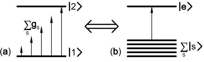
Figure 2.1: (a) The two-level atom interacting with a set of electromagnetic field modes. (b) When the atom is initially in the excited state and couples to the ground state via an ensemble of vacuum modes the system is equivalent to semi-classical photoionisation to a continuum.

Rabi-oscillations have been observed at microwave frequency using rubidium atoms highly excited into Rydberg states [41].

For transitions at optical frequencies however, it is observed that an excited atom will rapidly decay into the lower atomic level. This is in contrast to the reversible population oscillations predicted by the single-mode model described above. We now turn to the problem of accurately modelling the real atomic dynamics of atoms with transitions at optical frequencies. We find that the discrepancy between the theory and experiment can be corrected by including the interaction of the atom with a continuum of field modes.

2.4 Weisskopf-Wigner Theory

(40)

2.4. WEISSKOPF-WIGNER THEORY 23

rate of decay can be deduced.

The Hamiltonian of a two-level atom interacting with a infinite set of field modes is given by

H =~_ω₁_σ₁₁₊~_ω₂_σ₂₂₊~X

s

ωsˆa†saˆs+~

X

s

gs(σ+ˆas+σ−ˆa†s), (2.18)

where we have removed the zero-point energy associated with each field mode. We now restrict the atom to the situation where only one photon is present in one of the field modes while the atom is in the ground state. The restricted basis can be written as

|s_i = _|1_iA⊗ |. . . ,0,1,0, . . .i, (2.19)

|e_i = _|2_iA⊗ |0,0, . . . ,0i, (2.20)

where s _∈ [0,_∞) labels which of the infinite set of field modes the photon is in. Within this basis the Hamiltonian becomes

H =~_ω₂_σ_ee₊~X

s

(ω1+ωs)σss+~

X

s

gs(σs++σs−), (2.21) where σs+ = |eihs|. This Hamiltonian describes an excited state, |ei, coupled to a infinite set of lower levels, _|s_i. The set of energy levels _|s_i represent the atom in the ground state with one photon of frequency ωs. Thus, we have transformed our

Hamiltonian into the form of a classical photoionisation problem. To take account of the infinite set of field modes we change the summation into a three dimensional integral over the density of states:

X

s

−→

Z

D(ω_s)d3ω_s. (2.22)

The integral is taken over all possible field modes. Here _D(ω_s) is the density of

states, which in free space is frequency independent, isotropic and is found to be

D(0) = 2V /(2πc)3_{. It is important to recall that the dipole coupling element is a} function of both the frequency and orientation of each field mode with respect to the atomic dipole moment. That is

g(ω_s) = p·ˆeωsωs

(41)

where θ is the angle between the atomic dipole and the polarisation of the field mode ω_s. Transforming into an interaction picture we get the form of a Hamiltonian

describing the coupling between a single bound state and an isotropic continuum of free space modes:

H =~

Z

∆sσssD(0)d3ω_s+~

Z

g(ω_s)(σ_s₊+σ_s

−)D(0)d3ω_s, (2.24)

where ∆s = ω1 −ω2 +ωs. We assume that the solution to the dynamics is of the

form

|ψ(t)_i=ce(t)|ei+

Z

cs(t)|siD(0)d3ω_s. (2.25)

This results in the infinite set of coupled equations for the time-dependent coeffi-cients:

˙

ce(t) = −i

Z

g(ω_s)c_s(t)D(0)dω_s, (2.26)

˙

cs(t) = −i∆scs(t)−ig(ω_s)c_e(t). (2.27)

We now formally integrate the equation (2.27) and substitute this into the differential equation (2.26). This transforms the two coupled differential equations into a single integro-differential equation for the coefficient ce(t). Once the angular integrations

have been performed we find

˙

ce(t) = −

p2 6π2_c3_~

0 Z ∞

0

dωsω3s

Z t 0

dt0ce(t0)ei∆s(t

0₋_t₎

. (2.28)

So far this equation is exact. However, we now note that for large values of ∆s

the time integral makes a vanishing contribution, varying approximately as _∝1/∆s.

Since only frequencies around resonance contribute significantly, we can make the approximation ω3

s =ω213 . Therefore ˙

ce(t) = −

p2_ω3 21 6π2_c3_~ 0

Z ∞

ω1−ω2

d∆s

Z t 0

dt0ce(t0)ei∆s(t

0₋_t₎

. (2.29)

When the integral over the detunings is evaluated we obtain

Z ∞

ω1−ω2

d∆sei∆s(t

0₋_t₎

=πδ(t0₋t) +i_P. (2.30) The term _P is a principle value integral that leads to an energy shift of the state

(42)

2.4. WEISSKOPF-WIGNER THEORY 25

with non-zero Rabi-frequency and is closely related to the Lamb shift in hydrogen [6, 17]. Normally the energy shift is very small and is absorbed into the definition of the natural frequency ω21. In fact, this is an elementary example of the method of renormalisation often used in quantum field theory. Evaluating the time integral we find that the decay rate of the excited state is

˙

ce(t) = −

p2_ω3 21

6πc3~₀ce(t). (2.31)

This is easily solved to give the observed exponential decay of the excited atomic state:

ce(t) = exp(−Γt/2)ce(0), (2.32)

where the spontaneous decay rate has the value

Γ = p 2_ω3

21 3π0~c3

. (2.33)

We note that the spontaneous decay rate of the excited state is proportional to the cube of the transition frequency. This explains why decay rates of the order 10Hz are possible at microwave frequencies, as opposed to 10MHz at optical frequencies. Spontaneous emission can also be reduced by decreasing the number of field modes present, as is often done by placing the atom in a high Q-factor cavity.

(43)

2.5 Master Equations

In practice the problem of determine the dynamics of an ensemble of multilevel atoms coupling to a continuum of field modes in arbitrary photon number states is quite intractable. In addition, often the motion of the atoms, and the associated collisional and Doppler broadening, should be included in the analysis. Generally, spontaneous emission is only one of several decoherence mechanisms present. A more straightforward, and approximate method of accounting for all the degrees of freedom of the ensemble must be found. We represent the interaction between an atom and its environment by forming the density matrix equation of motion:

˙ˆ

ρ=₋i

~[ ˆH,ρˆ]−−Dˆ(ˆρ(t)), (2.34)

where ˆDis the decoherence operator. Our choice of decoherence operator depends on the decay and dephasing mechanisms which we expect to be present in the system, and the ease by which the resulting differential equations can be solved. One of the most general forms of decoherence operator is the Lindblad form [42]

ˆ

D(ˆρ(t)) = 1 2

X

m

γm

[ˆρLˆ†_m,Lˆm]−+ [ ˆL†m,Lˆmρˆ]−

. (2.35)

Hereγmgives the rate of each decay or dephasing process described by the operators

ˆ

Lm. For example, a spontaneous emission from an atomic level|2ito|1iis generated

by the operator ˆL =σ12. Similarly, a pure dephasing between two atomic levels is represented by ˆL = _√1

2(σ22−σ11). Such a dephasing could occur due to an elastic collision between atoms.

However, an alternative form of decoherence operator also exists, which although less general, produces a master equation that is much easier to solve. This master equation is

˙ˆ

ρ(t) = ₋i

~[ ˆH, ρ(t)]−−

1

(44)

2.5. MASTER EQUATIONS 27

atomic transitions, cannot be included by this mechanism. Similarly, no account can be made for the drift of atoms in and out of the interaction region. This is particularly significant for systems such as the atomic lambda system, which contains a pair of nearly degenerate ground states. According to the Maxwell-Boltzmann distribution there will be an appreciable probability for the atom occupying either ground state. Therefore, in a thermal gas there will be a constant drift of coherently prepared atoms out of the laser beam, and a drift of (almost maximally) mixed states into the interaction region. However, given a sufficiently low density gas (few collisions, with buffer gas present) prepared at low temperature (lower drift rate, less mixing and fewer collisions), it is possible to model an atomic system accurately using the master equation (2.36). This is particular significant since solutions to this equation are much easier to derive than solutions using the full Lindblad method. Consider the Schr¨odinger equation, where the Hamiltonian is no longer necessarily Hermitian:

∂

∂t|ψi=− i

~Hˆ|ψi, ≡

∂

∂thψ|=− i

~hψ|Hˆ

†_. _(2.37)

If we form the density matrix equation of motion ˆρ=_|ψ_ihψ_|, we find ˙ˆ

ρ=₋i

~

ˆ

Hρˆ₋ρˆHˆ†. (2.38) Now, we choose the non-Hermitian Hamiltonian to be of the form

ˆ

H = ˆHo−

i~

2Γˆ, (2.39)

where ˆΓ is represented by the diagonal decay matrix given above. Then we can rewrite the density operator equation of motion as

˙ˆ

ρ=₋i

~[ ˆHo,ρˆ]−−

1

2[ˆΓ,ρˆ]+. (2.40) Clearly, this is exactly the same form as the master equation given above (2.36). By solving the Schr¨odinger equation and making the substitution (2.39), where the eigenvalues of ˆHo become complex, we have also formed solutions to the master

(45)

decay can be understood as modifications to the real and imaginary parts of the eigenenergy of the excited state. In addition, as was shown in section 1.3 there exists a relationship between the Hamiltonian and the electric susceptibility. Thus, the Kramer-Kr¨onig relations between the real and imaginary parts of the susceptibility at least suggest that a similar relationship may exist for the transition energies.

One further caveat of the simple master equation (2.36) is that although it can model decay and decay induced dephasing, it cannot produce a cascade of population between energy levels. A very simple example of this is given by a system for which the matrix representation of the Hamiltonian is diagonal. In this case the diagonal elements of [H, ρ]₋ vanish and their evolution is dictated by the decay only:

˙

ρpp(t) =

−1

2[Γ, ρ(t)]

pp

=₋Γppρpp(t). (2.41)

The solution is given by the exponential decay ρpp(t) = exp(−Γppt)ρ(0). That is,

the population that decays from each atomic level is simply “lost” from the system and does not cascade. We interpret this as the atom spontaneously decaying into a state outwith our Hilbert space. The decaying behaviour is exactly that predicted by the Weisskopf-Wigner theory, although in many case the actual rate will vary significantly from the W.-W. result. This is due to multilevel effects that arise when energy levels are nearly degenerate and the simple two-level model presented above is no longer valid [36].

2.6 Electromagnetically Induced Transparency

(46)

[image:46.612.210.415.79.242.2]

2.6. ELECTROMAGNETICALLY INDUCED TRANSPARENCY 29

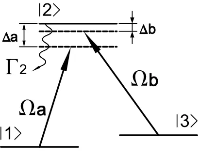
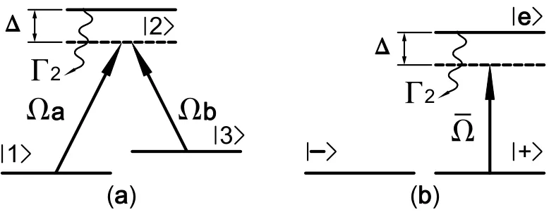
Figure 2.2: The atomic lambda system (Λ-system). Two ground states are coupled to a single excited state that decays at the rate Γ2.

to occur. More recently, the realisation that intra-atomic quantum interference can produce dramatic effects has been exploited in the phenomena of electromagnetically induced transparency (EIT).

It is well known that a classical electromagnetic field interacting with a quantum-mechanical two-level atom will experience a Lorentzian absorption profile. That is, the electric susceptibility for a density of N/V atoms in the ground state is given by [39]

χ(∆) = Np 2

~₀_V

∆ +iγ

∆2 ₊_γ2, (2.42)

where ∆₋iγ is the complex detuning predicted by the Weisskopf-Wigner theory. However, there is nothing particularly quantum-mechanical about this result. In fact the same response can be derived by considering the electron as a point charge trapped within a damped harmonic oscillator [17]. The true quantum-mechanical nature of bound-state electrons only becomes manifest when multiple excitation pathways exist and quantum interference can occur. This is analogous to interference occurring in the double-slit experiment.

(47)

consider the dressed states of the Hamiltonian [45]. Working within an interaction picture and for a semi-classical approximation (or when we restrict ourselves to within one resonant manifold [38]) the Hamiltonian has the matrix representation

H =~



   

0 Ωa/2 0

Ωa/2 ∆a Ωb/2

0 Ωb/2 ∆a−∆b



   

, (2.43)

where Ωα, α ∈ {a, b} are the Rabi-frequencies of both fields and ∆a = ω2 −ω1 −

ωa,∆b =ω2−ω3−ωb are the detunings. The characteristic polynomial that defines

the eigenvalues (En =~λn) is

4λ3₋4λ2(2∆a−∆b)−λ

Ω2_a+ Ω2_b ₋4∆a(∆a−∆b)

+ (∆a−∆b)Ω2 = 0. (2.44)

The eigenvalues can be found by depressing the cubic polynomial and then using a cosine substitution [36]. However, it is more instructive to consider the situation when the fields are Raman-resonant with the two photon transition between the ground states (∆a−∆b = 0). Then the eigenvalues are easily found to be

λD = 0, λ± = 1 2

∆a±

q ∆2

a+ ¯Ω2

, (2.45)

with ¯Ω2 _{= Ω}2

a+ Ω2b. The corresponding eigenstates are

|D_i = 1_¯

Ω(Ωb|1i −Ωa|3i), (2.46)

|Φ_±_i = 1

N_±(Ωa|1i+ Ωb|3i+ 2λ±|2i). (2.47)

The eigenstate _|D_i is called the dark state of the Λ system. It is non-interacting, or dark, to the electromagnetic fields since the density matrix elements ρ21 and ρ23 vanish. This can be explained by the destructive interference between excitation from both ground states. That is, the population is shared among the ground states so as to maintain balanced but anti-phase excitations.

(48)

2.6. ELECTROMAGNETICALLY INDUCED TRANSPARENCY 31

-2 -1 0 1 2

Da

-0.5 0 0.5 1

Χ

H

1

L HΩ

a

;

Ωa

L

Ha_L

-2 -1 0 1 2

Da

-0.5 0 0.5 1

Χ

H

1

L HΩ

a

;

Ωa

L

[image:48.612.124.502.73.195.2]

Hb_L

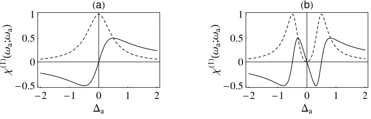
Figure 2.3: The form of the linear electric susceptibilities for (a) two-level atom and (b) the atomic lambda system.

Λ-atoms can be rendered transparent by the addition of a second Raman-resonant field and the subsequent relaxation into the dark state.

This procedure is called electromagnetically induced transparency (EIT) and was first suggested in 1989 by Harris and Imamoˇglu [46] when investigating the possibility of lasing without inversion (LWI). Since then the field of gas-phase nonlinear optics has flourished due to the creation of several successful and promising EIT based schemes. In practice transparency is usually achieved in an atom illuminated by one weak (Ωa) and one strong (Ωb) field. These are usually named the probe and

pumpfields respectively. Within this approximation the linear electric susceptibility experienced by the probe field is

χ(1)(ωa;ωa) =

4N(∆a−∆b)|p12|2

~₀_V _[4(∆_a₋_∆_b_)(∆_a₋_iγ₁₎₋_Ω2

b]

. (2.48)

This electric susceptibility is compared with the two-level case in Fig.(2.3). We note that due to the presence of the atomic dark-state on resonance, the Lorentzian absorption profile has been split into two components. These are called the Autler-Townes components and were observed by spectroscopic analysis of an optically thin gas in 1955 [47].

(49)

then it has been proposed that slow-light, ordark-state polaritons[49], could be used to stop and store light pulses to form an optical quantum memory [50]. Indeed, there has already been considerable success in storing light pulses in both rubidium vapour [51], doped solids [52] and even at the single photon level [53].

(50)

Chapter 3 Steady-State Cross-Phase

Modulation

In chapter 1 it was demonstrated that cross-phase modulation will occur in any non-linear centrosymmetric classical material. However, by using coherent interactions between light and an ensemble of atoms it is possible to produce a much stronger, and often pure cross-phase modulation. This possibility was first explored when considering the three-level atom in the EIT configuration. The Λ configuration does however have serious limitations which will be discussed below. Nonetheless, by modifying this system to include a fourth atomic level we are able to overcome many of these problems.

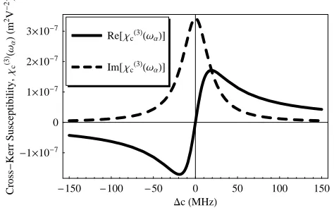
The possibility of achieving large cross-Kerr nonlinearities in the four-level atom, known as the N-configuration atom, was first suggested by Schmidt and Imamoˇglu in 1996 [54]. It is the investigation of this system in the non-resonant [59, 60] and time-dependent regimes [61] that constitutes my original work in this thesis. Recently it has been suggested that equally strong nonlinearities could also be produced in the Λ atom by using a single-mode cavity to enhance the interaction [62]. This interesting development has yet to be experimentally realised, but appears to provide another viable method for the generation of large XPM in atomic systems.

(51)

34 CHAPTER 3. STEADY-STATE CROSS-PHASE MODULATION

3.1 XPM in the

Λ

_System

To show that cross-phase modulation can be produced in a Λ atom we begin by working in the EIT limit. In this case the ground states of the Λ atom are coupled to the excited state by the pump (Ωb) and probe fields (Ωa), see fig. 2.2. The electric

susceptibility experienced by the weak probe field Ωa is

χ= 4N(∆a−∆b)|p12| 2

~₀_V _[4(∆_b ₋_∆_a_)(∆_a₋_iγ₎₋_Ω2

b]

. (3.1)

Here, the susceptibility has been calculated to first-order in Ωa and to all orders in

Ωb. We now make the approximation that the control field Ωb is strongly detuned,

in particular we have Ωb (∆b −∆a)(∆a−iγ). Then the susceptibility can be

Taylor expanded in Ωb to give linear and XPM terms:

χ(1)(ωa;ωa) =

N_|p12|2

~₀_V_(∆_a₋_iγ₎, (3.2)

χ(3)₍_ω

a;ωa, ωb,−ωb) =

N_|p12|2|p34|2 4~3_V_(∆

a−iγ)2(∆a−∆b)

. (3.3)

The linear term is found to be the usual Lorentzian absorption for an atom in the ground state and the nonlinear term is the cross-phase modulation which we required (Fig. 3.1). However, this configuration has a serious drawback: the XPM is maximal when the probe field is close to resonance with the Lorentzian absorption peak (see fig.(2.3a)). The essential problem of with XPM in the Λ atom is that the XPM is obscured by strong Lorentzian absorption. Unfortunately this cannot be mitigated by working off-resonance since the XPM term decays faster than the linear absorption.

Recent demonstrations of the XPM generated in the three-level atom have chosen to operate on resonance of the probe field [63]. In this case the nonlinear suscepti-bility simplifies to

χ(3)(ωa, ωa, ωb,−ωb) =

4N_|p12|2|p23|2

~3_{V γ}2_∆

b

. (3.4)

Cross phase modulation in rubidium 87

Cross-Phase Modulation in Rubidium-87

Gary F. Sinclair

PhD Thesis

School of Physics and Astronomy,

University of St Andrews,

St Andrews,

United Kingdom

26

Contents

Abstract

Declarations

Publications and Conferences

Journal Publications

Conference Presentations

Acknowledgements

Introduction

Chapter 1

Introduction to Quantum Optics

1.1

Classical Electrodynamics

1.1.1

The Maxwell Equations in Dielectric Media

1.1.2

The Electric Dipole Interaction

1.2

Field Quantisation

1.2.1

The Electromagnetic Field Hamiltonian

1.2.2

Quantum States of the Field

1.3

Nonlinear Dielectrics

1.3.1

Classical Description

1.3.2

Quantum-Mechanical Description

Chapter 2

Introduction to Quantum

Electronics

2.1

The Schr¨

odinger Equation

2.2

Interaction Pictures

2.3

Dressed States

2.4

Weisskopf-Wigner Theory

2.5

Master Equations

2.6

Electromagnetically Induced Transparency

Chapter 3

Steady-State Cross-Phase

Modulation

3.1

XPM in the

Λ

System

_System