Evaluation of formability and fracture of pure titanium in incremental sheet forming

ORIGINAL ARTICLE

Evaluation of formability and fracture of pure titanium

in incremental sheet forming

Shakir Gatea1&Dongkai Xu2&Hengan Ou1&Graham McCartney1

Received: 25 June 2017 / Accepted: 6 October 2017

#The Author(s) 2017. This article is an open access publication

Abstract A forming limit diagram (FLD) is commonly used as a useful means for characterising the formability of sheet metal forming processes. In this study, the Nakajima test was used to construct the forming limit curve at necking (FLCN) and fracture (FLCF). The results of the FLCF are compared with incremental sheet forming (ISF) to evaluate the ability of the Nakajima test to describe the fracture in ISF. Tests were carried out to construct the forming limit diagram at necking and fracture to cover the strain states from uniaxial tension to equi-biaxial tension with different stress triaxialities—from 0.33 for uniaxial tension to 0.67 for equi-biaxial tension. Due to the fact that the Gurson–Tvergaard-Needleman (GTN) model can be used to capture fracture occurrence at high stress triaxiality, and the shear modified GTN model (Nahshon-Hutchinson’s shear mechanism) was developed to predict the fracture at zero stress or even negative stress triax-iality, the original GTN model and shear modified GTN model may be not suitable to predict the fracture in all samples of the Nakajima test as some samples are deformed under moderate stress triaxiality. In this study, the fractures are compared using the original GTN model, shear modified GTN model and the Nielsen-Tvergaard model with regard to stress triaxiality. To

validate the ability of these models, and to assess which model is more accurate in predicting the fracture with different stress triaxialities, finite element (FE) simulations of the Nakajima test were compared with an experimental results to evaluate the applicability of the Nakajima test to characterise the frac-ture from ISF. The experimental and FE results showed that the shear modified GTN model could predict the fracture ac-curately with samples under uniaxial tension condition due to low stress triaxiality and that the original GTN model is suit-able for an equi-biaxial strain state (high stress triaxiality), whereas the stress triaxiality modified GTN model should be considered for samples which have moderate stress triaxiality (from plain strain to biaxial strain). The numerical and exper-imental FLCF of pure titanium from the Nakajima test showed a good agreement between the experimental and numerical results of ISF.

Keywords Nakajima test . ISF . FLD . Stress triaxiality . GTN model

1 Introduction

It is important to predict the fracture and forming limits during the process in sheet metal forming processes. The forming limit diagram (FLD) of SPIF is usually employed to determine the limits of proportional straining before failure and is quite different from the corresponding diagram for traditional sheet forming such as deep drawing or hydroforming. The experi-mental results showed that the distribution of the thickness is uniform in the cross-section of the parts produced by ISF up to the fracture without necking before the fracture. Based on these results, the forming limit curve at necking (FLCN) of traditional sheet metal forming is not suitable for ISF. Consequently, the forming limit curve at fracture (FLCF) is * Shakir Gatea

Shakir.Gatea@nottingham.ac.uk * Hengan Ou

H.Ou@nottingham.ac.uk

1

Department of Mechanical, Materials and Manufacturing Engineering, Faculty of Engineering, University of Nottingham, Nottingham NG7 2RD, UK

utilised to predict the fracture of the ISF process [1]. The shape of the FLCF is a straight line with a negative slope for most of the materials and it is located in the first quad-rant of the forming limit diagram. Figure 1 illustrates the typical modes of deformation when a sheet element is subjected to proportional loading. In Fig. 1, the forming limit curves FLCN and FLCF are stated as a strain ratio of the true minor strainε2to the true major strainε1,

ρ=ε2/ε1and this ratio takes different values for different paths

of strain, e.g.ρ= 1for biaxial tension andρ= 0for plain strain [2–4].

Allwood et al. [1] proved that the formability of ISF is higher than that for conventional sheet metal forming by com-paring between them using a paddle forming process with the same geometry. They noted that the forming limit of ISF is increased under uniform proportional load when through-thickness shear is presented. Forming parameters, e.g. type of material, shape produced, tool diameter and step size, play an important role in increasing or decreasing the forming limits in SPIF [5]. A new forming tool containing a rotating ball was developed by Shim and Park [6] to evaluate the formability of Al 1050; in their study, different tool paths were applied to generate different strain paths. It was noted that formability was strongly influenced by the strain path. Jeswiet and Young [7] developed FLD for ISF of 5754–0 and 3003–0 Al using five distinct shapes to measure the major and minor strains at different status-es. It was found that, with SPIF, the strain increased over 300% for all shapes. An experimental methodology was then proposed to determine the FLCF using a SPIF, torsion and shear test. It is noted that the FLCF con-structed by a conventional sheet test, e.g. the Nakajima test, is identical to that constructed from ISF tests on pyramidal and conical truncate parts [8]. The major strain at fracture in ISF was located above the Nakajima’s forming limit curve at fracture (FLCF) when lower tool dim-eter is used [9].Tensile and hydraulic bulge tests were utilised to establish the FLCF for multi-stage SPIF. The results

showed that the FLCF can be successfully employed to deter-mine the forming limit of multi-stage SPIF. In addition, the overall strains obtained in multi-stage SPIF are higher than the FLCN established by the hydraulic bulge test [10]. The defor-mation mechanism and fracture behaviour of double point incremental forming has been investigated based on the mem-brane analysis and experimental work. It was found that by using different supporting force and tool shift the FLCF can be increased as compared with SPIF [11]. An analytical model was developed with the consideration of bending effect and strain hardening to describe the localised deformation in ISF. The results of this model showed that the deformation in ISF occurs in contact area as well in the neighbouring wall [12]. Stress-based forming limit diagram combined with maximum shear stress diagram criterion was introduced to predict the fracture in ISF process. This approach showed a good corre-lation between the prediction and experimental data [13]. The FLCF was constructed under proportional loading (tensile test) and non-proportional loading (SPIF test). It was found the shape and value of FLCF in SPIF differ from the one of tensile test [14].

To investigate the effect of friction on the formability and material deformation of SPIF, a new oblique roller ball (ORB) tool has been developed by Lu et al. [15]. Four grades of aluminium sheets were employed in the experiments includ-ing AA110, AA2024, AA5052, and AA6111. A small hole in the sheet was drilled to study material deformation under both traditional rigid tool and the ORB tool. Experimental results showed that higher formability and smaller through-thickness shear are obtained with the ORB tool. Modified Mohr-Coulomb (MMC) damage model was implemented in Abaqus/Explicit via user subroutine (VUMAT) to pre-dict the ductile fracture in SPIF. According to the Lode angle parameter and stress triaxiality, it was found the loading path of SPIF is non-linear as well, the MMC model with non-linear damage accumulation can predict the SPIF fracture location accurately while there was 10% error in fracture depth prediction [14]. An analytical model has been developed with the consider-ation of strain hardening and bending to study the de-formation stability and fracture in ISF process of alu-minium grads, AA1100 and AA5052. It was found the bending mechanism has a significant effect on the de-formation stability as well as the fracture occurs based on the material’s ductility and deformation stability [16]. FE simulation was employed to analyse the deformation of SPIF. The results showed that the SPIF part deforms under three deformation modes, i.e. stretching, shearing and bending [17].

region (left hand side) of FLD, although the prediction was not accurate in the tension-tension region (right hand side) of FLD. The original GTN model was utilised by Uthaisangsuk et al. [19] to simulate the FLD and forming limit stress dia-gram (FLSD). The investigation showed that the FLD was not suitable for the complex sheet metal forming process and that, with a multi-step forming process, the FLSD is more accurate than the FLD. Furthermore, the original GTN model showed acceptable prediction of the fracture. The original GTN model was employed by Parsa et al. [20] to predict the FLD for aluminium monolayer and sandwich sheets. The results showed a good correlation between the experiments and the original GTN model, especially in a biaxial strain state, due to the high stress triaxiality ratio created by this state. The Nakajima test was carried out by Min et al. [21] to plot the FLD and FLSD for an aluminium alloy (AA) 5052-O1 sheet. The fracture in the Nakajima test was predicted using the original GTN model, which showed good agreement with the experimental Nakajima test for all strain states. The original anisotropic GTN model was implemented in ABAQUS/Explicit by Kami et al. [22] to construct the FLD of an anisotropic aluminium sheet using the Nakajima test. The result of the original anisotropic GTN model showed a better correlation with the exper-imental Nakajima test, especially in the biaxial tension strain state. The ductile damage in ISF of pure Ti sheet was investigated numerically using shear modified GTN damage model. There was a good correlation of the fracture depth when the shear modified GTN model re-sults were compared with the experimental ISF test [23].

It is clear from the literature that the original GTN model has been used to simulate the Nakajima test in order to con-struct the forming limit curve at necking. The results showed that there was a good correlation between the FE prediction and experiments, especially in the biaxial strain state (high stress triaxiality) [20,22] due to the high stress triaxiality ratio created by this state. It also clear that the ability of the Nakajima test to describe the fracture in ISF is still debatable; some researchers claim that the test is iden-tical to that constructed from ISF tests on pyramidal and conical truncate parts [8], while others proved that the major strain at fracture in ISF is located above the Nakajima’s FLCF when a small tool dimeter is used [9]. In this study, for the first time, the GTN damage model with consideration of stress triaxiality has been employed to construct the forming limit curves at frac-ture in the Nakajima test and in incremental sheet forming at moderate stress triaxiality. To evaluate the ability of stress triaxiality modified GTN damage model and to predict the fracture under different stress strain states, the results were validated by Nakajima and ISF experimental results. In addition, the results of the

FLCF of Nakajima test are in a good agreement with that from ISF, which indicates the suitability of applying the Nakajima test to describe the fracture in ISF.

2 GTN model

The Gurson model [24] was developed based on the assump-tion that the material has a spherical shape of voids in the matrix. This model was modified by Tvergaard-Needleman [25] and the modified yield surface is defined as

∅¼ σq

σy 2

þ2q1f*cosh −

3q₂p 2σy

− 1þq3f*

2

¼0 ð1Þ

where σq¼

ffiffiffiffiffiffiffiffiffiffiffiffiffi

3 2SijSij

q

is the equivalent stress of the Von

Mises;σyis the flow stress;q1,q2andq3are the constitutive

parameters proposed by Tvergaard [26] with suggested values ofq1= 1.5, q2= 1.0andq3¼q21,p¼−13σiiis the hydrostatic

stress.f∗was proposed by Tvergaard-Needleman [25] to eval-uate the coalescence between the voids and is given by

f*¼

f if f≤fc

fcþ f_F−f_c

f_f−fc ðf−fcÞ if fc< f < fF

f_F if f≥f_F

8 > > < > >

: ð2Þ

wherefcis the critical value of the void volume fraction;fFis

the void volume fraction at fracture, andf_F is given by:

_f

F ¼

q₁þ ffiffiffiffiffiffiffiffiffiffiffiffiq2 1−q3

p

q₃ : ð3Þ

In the original GTN model, the void volume fraction is increased under tensile loading, due to the growth of the existing void and based on the nucleation of the new void.

f_total¼df_nucleationþdf_growth ð4Þ

The increment of the void nucleation is described by:

df_nucleation¼Adεp_m ð5Þ

where A¼ f_N SN ffiffiffiffiffiffi 2π p e−0:5

dεpm−εN SN

2

if p≥0

0 if p<0:

2 6 6

4 ð6Þ

The parameterAis a function of the matrix of total equiv-alent plastic strain εp

m,fNis the void volume fraction of the

nucleated void;εNis the mean value of the normal distribution

of the nucleation strain; andSNis the standard deviation.dεp_m

The increment of void growth is defined by:

dfgrowth¼ð1−fÞdε

p

ii ð7Þ

wheredεp_iiis the trace of the plastic strain tensor.

When the shear loading is considered, the shear load can accelerate the growth of the void or nucleate the new void. Therefore, the original GTN model was modified by Nahshon and Hutchinson [27] by adding an extension to predict the rate of the growth of voids with low stress triaxiality.

df_shear¼kwfω σ_σð Þ

q

S:ε˙p _ð8Þ

whereω(σ) is a function of the stress state and its value is calculated as:

ω σð Þ ¼1− 27J3 2σ3

q

!2

: ð9Þ

The range ofωis between 0≤ω≤1 with all axisymmetric stress statesω= 0and for all the states of pure shear plus a hydrostatic contribution ω = 1. kw is a parameter

pro-ducing the damage rate in shear loading, and J3 is the

third invariant of the deviatoric stress tensor J3= det(S).

In shear modified GTN model the increment of the VVF is determined based on the micro-voids’ nucle-ation, growth and shear mechanisms.

The shear modified GTN model is able to predict fracture under very low stress triaxiality (ƞ), while the original Gurson model predicts the fracture under high stress triaxiality. Therefore, Nielsen and Tvergaard [28] modified the Nahshon and Hutchinson shear extension to cover the effect of stress triaxiality in the regions of moderate to high stress triaxiality. Therefore, the function of the stress state becomes

ωo¼ω σð ÞΩð Þƞ ;withΩð Þƞ

¼

1_ƞ;_−ƞ for ƞ<ƞ1 2

ƞ1−ƞ2

; for ƞ₁≤ƞ≤ƞ₂

0; for ƞ>ƞ₂

2 6 4

ð10Þ

whereω(σ) is given by Eq. (9),ƞ1<ƞ2; based on this addition,

the original GTN model is used forƞ>ƞ2and the shear

mod-ified GTN model is utilised forƞ<ƞ1.

3 Experimental works

3.1 Nakajima test

This test is a stretching process up to fracture and is used to predict the forming limit diagram. The tools used in this test

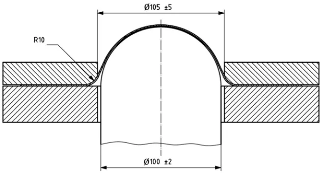
include a hemispherical punch, die, and blankholder. Figure2 shows the Nakajima test configuration according to BS EN ISO 12004-2. The spark-erosion method is utilised to produce the final shape of the specimen because it does not cause cracks in the sample’s edges.

More than one specimen is required for the description of a complete forming limit diagram from uniaxial to equi-biaxial tension. In this work, five geometries of pure Ti grade1 with a sheet thickness of 0.7 mm were examined with three repeti-tions. The sample dimensions are illustrated in Table1 and Fig.3. Prior to the formability test, acetone was used to clean the sample, after which grease and PVC of 1 mm thickness were applied to the contact surface as a lubricant to reduce friction between the punch and specimen. The test was with a punch velocity equal to 1.2 mm/s.

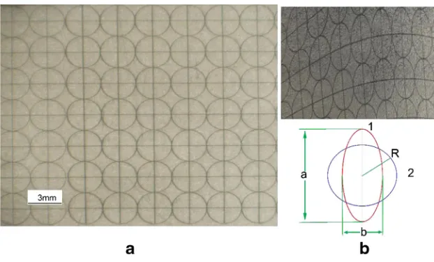
The technique utilised for obtaining the forming limit curve at necking (FLCN) included using electrical chemical etching to print a grid of circles with a 2.5-mm initial diameter on the surface before the stretching process, and to measure the ma-jor and minor axis dimensions of the ellipses that resulted from the plastic deformation. The values of strain are comput-ed from Eq. (11) (see Fig.4) [29]:

εmajor¼ln

a

do ;εminor ¼

ln b

do ð

11Þ

wheredorepresents the original diameter of the circle anda

andbare the major and minor axes of the ellipse.

In addition, the optical deformation measurement with the digital camera was used to evaluate the major and minor strain distributions on the outer surface of the blank. The procedure for establishing the FLCF began by measuring the thickness at fracture in several places along the crack in order to obtain the average thickness strain. Average thickness strain was evalu-ated on both sides of the fracture. By using the grid pattern, the average minor strain was evaluated along the fracture, and by using volume constancy, the major strain was determined as follows:

εmajor¼−ðεminorþεthicknessÞ ð12Þ

3.2 Determination of mechanical properties and GTN model parameters of pure titanium

image was analysed using ImageJ to determine the primary VVF (fo). The same technique was applied to determine the

values of the VVF at nucleation, critical and fracture. The value for nucleation in the VVF (fN) is determined when

plas-tic deformation occurs in the tensile sample and before reaching the maximum load. It is difficult to predict the load where nucleation begins; therefore, the tensile test was stopped at different stages in order to scan the sample to de-termine whether nucleation had started. In this study, nucle-ation started when the load reached 2.8 kN. When the tensile sample reached the maximum value of the force and necking was noticed, the tensile test was stopped to determine the critical value of VVF (fc). Finally, the fracture surface of the

tensile sample was scanned using SEM to determine the final value of VVF (fF). Table2summarises the mechanical

prop-erties and the GTN model parameters of pure Ti grade 1.

3.3 Single-point incremental forming

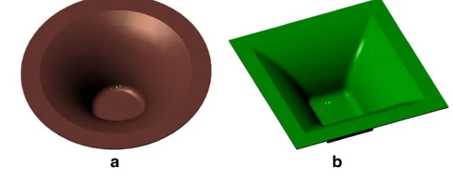
The proposed experimental method to establish the forming limit curve at fracture makes use of SPIF. The SPIF test was carried out to form truncated conical and pyramidal geome-tries with varying forming angles from 22° to 80°, as shown in Fig.6. The truncated cone and truncated pyramid allow con-struction of the FLCF directly from the experimental measure-ment of major and minor strains at fracture under plain strain

and biaxial stretching conditions. To measure the strain state, the circle grid analysis was utilised using a similar methodol-ogy to the Nakajima test.

These tests were done with an incremental depth equal to 0.2 mm per revolution and tool diameter of 10 mm. The tool is rotation free with a feed rate of 1000 mm/min. To ensure the repeatability of the results, the SPIF process was repeated three times and the average value was taken.

4 Finite element simulation

Abaqus/Explicit was used to implement the shear modified GTN and stress triaxiality modified GTN models as a mate-rials user subroutine (VUMAT). A return mapping algorithm was then utilised to determine the increments in plastic strain (dεp

) [30,31]. Figure7shows the FE model of the Nakajima test performed on a specimen with a width ofa= 90 mm and SPIF. In the simulation of the Nakajima test, the punch, die and the blankholder were modelled as an analytical rigid sur-face. This was the same for the tool, the backing plate and the blankholder in the SPIF process. The blank was modelled as a deformable body with an eight node brick element (C3D8R) in both the Nakajima test and the SPIF process. Element de-letion technique was used to remove the failed elements from Fig. 2 Illustration of the cross

section of the tool used for Nakajima testing [ISO 12004-2]

Fig. 3 Dimensions of different FLD samples prepared for experiments Table 1 The dimensions of Nakajima test specimens

Parameters Sample 1 Sample 2 Sample 3 Sample 4 Sample 5

the FE model and to model the fracture in the sheet. In FE simulation, velocity vs time was used to define the tool path in SPIF and the movement of the punch in the Nakajima test.

The Nakajima test was carried out in two steps. In the first step, a 50-kN holding force was applied to the reference point of the blankholder. In the second step, the holding force remained constant and the punch moved down in the vertical direction. In this investigation, the Nakajima test was run five times with different dimensions, as shown in Table1, to cover a uniform distribution of the FLC from uniaxial to equi-biaxial tension. Minor and major strains were recorded at the end of each job corresponding to a point on the FLD.

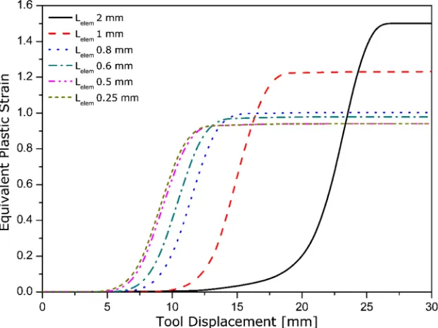
To study the effect of simulation parameters on the FE results, 45° truncated cone is executed with a 116-mm major base and a final depth of 30 mm. The SPIF test is carried out with a 10-mm hemispherical forming tool and 0.2-mm step size with a 1000 mm/min feed rate. Meshing density has an effect to the simulation results. However, using a very small element size means that the computational time be increased due to the fact that a stable increment time is strictly dependent on the element’s length for explicit integration. In order to study the optimum mesh size to accurately predict the fracture with GTN model simulation of Nakajima test and SPIF, six element lengths (2, 1, 0.8, 0.6, 0.5 and 0.25 mm) were chosen

with three layers of elements through the thickness. In this work, equivalent plastic strain distribution is used to predict a suitable element size. Figure8shows the equivalent plastic strain distribution of SPIF with different mesh sizes. It is clear from the figure that with a smaller element size, the increment in equivalent plastic strain can be captured earlier than that with larger element sizes. It can be concluded that using a solid element with reduced integration means each element has one integration point in the middle; hence, if a large ele-ment is used, the possibility of capturing the peak of the equiv-alent plastic strain is less than when using a small element. In this investigation, therefore, an optimum element size of 0.5 mm was chosen for this investigation.

To check the validity of the SPIF simulation, the FE thick-ness was compared with experimental SPIF thickthick-ness, as shown in Fig.9. The SPIF simulated results by Abaqus are consistent with one of the actual experiments.

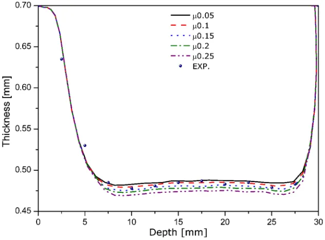
In most sheet metal forming processes, low friction is favoured. In the SPIF process, a certain level of friction is required between the forming tool and the sheet to transfer the stresses onto the forming tool and allow some stretching of the sheet. In order to investigate the effect of friction on the FE model of the SPIF process, the contact between the tool and blank, was simulated with different values of friction co-efficient (μ= 0.05, 0.1, 0.15, 0.2, and 0.25). The predicted thickness was compared with that of the experiment to illus-trate the effect of friction coefficient on thickness distribution, as shown in Fig.10. It can be seen that there is a good corre-lation in the thickness distribution of the truncated cone be-tween the simulation results of a 0.1 friction coefficient and the experimental thickness. Hence, friction coefficient,μ= 0.1 is chosen in this work to simulate the friction in SPIF between the forming tool and the sheet. It is clear therefore that more

thinning can be achieved with a high friction coefficient (μ= 0.25).

In Nakajima test, the friction should be controlled to get accurate results of forming limit diagram. According to the BS EN ISO 12004-2:2008, the Nakajima test is considered valid if the fracture takes place with a distance less than 15% of the punch diameter away from the centre of the dome. The occur-rence of the fracture away from the apex of the dome gives Indicator a high value of friction between the punch and blank [3]. The specimen with widtha= 90 mm was chosen to study the effect of friction coefficient on the predicted fracture loca-tion. In the FE simulation, the friction coefficient between the pure Ti sheet and the punch was set to four valuesμ= 0.25, 0.15, 0.1 and 0.05. Figure11shows the effect of friction co-efficient on the fracture locations. It is clear from the figure with the high values of friction coefficient (0.25 and 0.15) the fracture occurs away from the apex of the dome with distance more than 15% of the punch dimeter and this distance gets smaller to be less than 15% of the punch diameter with 0.1 friction coefficient and very near to apex of the dome with 0.05 friction coefficient. A 0.05 friction coefficient is chosen in this work to simulate the friction between the punch and blank in Nakajima test and with this value a good correlation was achieved between the FE simulation and experimental test.

5 Results and discussion

5.1 Nakajima test

The level of major strain at fracture in different strain states is illustrated in Fig.12. It is evident that relatively high major

Fig. 6 Geometries which require establishing FLD by using SPIF.a Cone.bPyramid

Table 2 Material properties and GTN model parameters of pure Ti

Yield stress Ultimate tensile stress Young’s modulus Poisson’s ratio Density fo q1 q2 fN εN SN fc ff

strain concentrations were present in the fracture zone of the stretched piece as a result of excessive bending.

Figure13illustrates the distribution of major and minor strains in all samples of the Nakajima test. From the figure, it can be seen that the ratio between the minor and major strain is−0.5,−0.11, 0.03, 0.901 and 1 for specimens with a width ofa= 20, 60, 90, 130 and 170 mm, respectively. Based on these ratios, the samples are enough to cover all strain states from uniaxial tension (strain ratio = − 0.5) to equi-biaxial tension (strain ratio = 1) and the specimens with a width of a= 20, 90 and 170 mm corresponded well to strain states of uniaxial tension, plain strain and equi-biaxial tension, respectively.

To describe the complete FLCN and FLCF, five geometries were used to cover all the strain states from uniaxial tension to

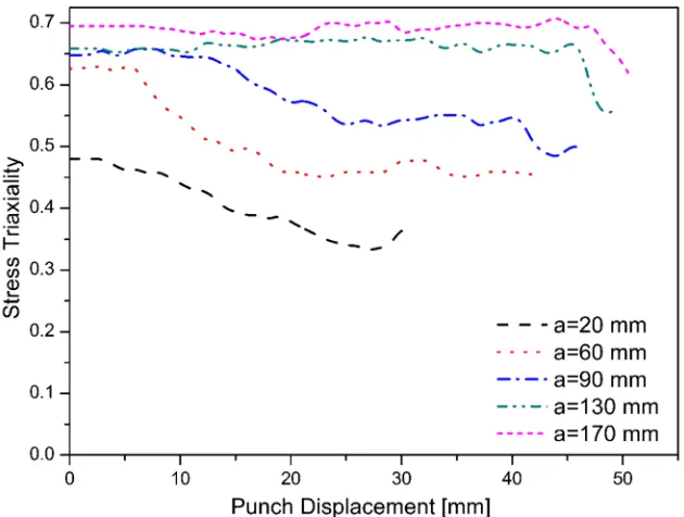
equi-biaxial tension and these samples experienced different stress triaxiality, as shown in Fig.14. From the figure, it is clear that stress triaxiality was not constant during the defor-mation of each sample. Therefore, the average value of stress triaxiality was taken as a reference of each sample and was 0.39, 0.5, 0.57, 0.63 and 0.66 for samples with a width of a = 20, 60, 90, 130 and 170 mm, respec-tively. Based on these results, stress triaxiality appears to change from one sample to another; in the Nakajima test, it also changed in the same sample. Therefore, the effect of stress triaxiality on the fracture occurrence should be taken into account when the GTN model is used to evaluate the fracture in the Nakajima test.

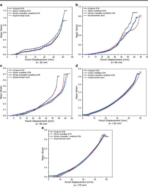
Major strain at fracture was measured using FE models (the original GTN, shear modified GTN and stress triaxiality

Fig. 8 Comparison of equivalent plastic strain between meshing densities of SPIF

modified GTN) and from experimental tests for all Nakajima samples to validate and examine these models. Figure15a shows the distribution of major strain on all FE models, as well as the experimental tests for samples with a width equal to 20 mm (uniaxial tension). It is clear from the figure that there is a good correlation between the shear modified model and experimental curve; this correlation is due to the fact that the value of stress triaxiality is normally considered low (0.39) and the Nahshon-Hutchinson’s shear mechanism was added to capture the fracture at low stress triaxiality, but the original GTN model cannot predict the void’s growth within this range

of stress triaxiality and coalescence is postponed. Specimens with a width of 60 and 90 mm have moderate stress triaxiality; therefore, both the original GTN model and shear modified GTN model cannot accurately predict the value of the major strain at fracture, as shown in Fig.11b, c; this is due to the fact that the original model and shear modified model do not work with a moderate ratio of stress triaxiality. However, the stress triaxiality modified GTN model is considered the best choice to use when moderate stress triaxiality is generated during the deformation as this model can accommodate the effect of stress triaxiality. The ratios of stress triaxiality in specimens

with widths of 130 and 170 mm are normally considered high at 0.63 and 0.66, respectively. With this range of stress triax-iality, the original GTN model can predict the fracture

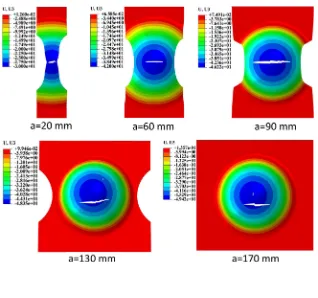
occurrence accurately, as shown in Fig. 11d, e). Therefore, based on the above results for processes under different stress triaxialities, e.g. the Nakajima test, it is better to use the GTN Fig. 11 Effect of friction

coefficient on the fracture location in Nakajima test

model which considers the range of stress triaxiality as the Nielsen-Tvergaard stress triaxiality extension of the GTN model can be used as either the original GTN model, the shear modified GTN model, or as a stress triaxiality modified GTN model.

The predicted fracture depth (FD) of Nakajima test with different widths was validated by the experimental depth, as shown in Figs.16and 17. It is clear that the fracture depth shows a good correlation between simulations using Abaqus/

Explicit with the stress triaxiality modified GTN model and the experimental measurements.

5.2 Single-point incremental forming

The stress triaxiality modified GTN model was used to simu-late the SPIF process for two shapes (hyperbolic truncated cone and hyperbolic truncated pyramid) due to the ability of this model to predict fracture occurrence with different stress

Fig. 14 Evaluation of stress triaxiality of Nakajima test specimens

triaxialities. The distribution of the major strain in SPIF parts is illustrated in Fig. 18. In the hyperbolic truncated cone

Fig. 17 Fracture depth of Nakajima test specimens with different widths

contact zones, whereas in the hyperbolic truncated pyramid, it is concentrated at the corner of the part.

The values of major and minor strains for both shapes were recorded, as shown in Fig.19, and the ratios of strain (ρ=ε2/

ε1) were 0.05 and 0.87 for the hyperbolic truncated cone and

hyperbolic truncated pyramid shape, respectively. These ratios were validated experimentally by measuring the major and minor strain at fracture in SPIF for both shapes. Figure20 shows the deformed grid at fracture; it is observed from the

diagram of the hyperbolic truncated cone shape that there is a big change on one axis of the circular grid, whereas the change in the other one is small, meaning there is an increase in major strain, while the minor strain remains unchanged (plain strain).It is also observed with the hyperbolic truncated pyra-mid shape that there is uniform distortion in the grid at fracture and that the ratio is close to 1 (equi-biaxial strain). Based on these ratios of strain, the hyperbolic truncated cone is de-formed under plain strain conditions and the corner of the hyperbolic truncated pyramid part is deformed under equi-biaxial strain. Therefore, two points can be recorded in the first quadrant of FLD; these points are used to validate the capability of the Nakajima test to describe the formability of SPIF process.

The values of major strain in both shapes were com-pared with the experimental SPIF test to validate the abil-ity of the stress triaxialabil-ity modified GTN model to accu-rately predict the values of major strain at fracture, as shown in Fig. 21. The results show that major strain in the hyperbolic truncated pyramid shape increases earlier than in the hyperbolic truncated cone due to the fact that the fracture develops in the corner of the hyperbolic pyr-amid shape under equi-biaxial stretching, whereas plain strain stretching appears in the hyperbolic cone shape. The SPIF-simulated results by Abaqus, using the stress triaxiality modified GTN model, are consistent with those of the actual experiments for both shapes. From the FE and experimental results, it is noted a higher fracture an-gle can be achieved with the hyperbolic truncated cone (68°) than the hyperbolic truncated pyramid (61°), this is due to the fact that the truncated cone deforms under

Fig. 19 Distribution of major and minor strain in both the hyperbolic truncated cone and hyperbolic truncated pyramid shape

plane strain stretching (minor strain close to zero), while the truncated pyramid deforms under the plane strain and equi-biaxial strain stretching (minor strain equal the ma-jor strain) with the equi-biaxial stretching greater than the plane-strain stretching. Therefore, a high degree of deformation can be achieved under the plane strain condition.

5.3 Forming limit diagram

The experimental Nakajima test was conducted at ambient temperature with specimens of widths 20, 60, 90, 130 and 170 mm; the test was stopped when a crack occurred in the

sample. The FLCN was established by measuring the major and minor strain in the necking region, while the FLCF was determined by measuring the major and minor strains in the fracture region and then plotting them in the major and minor strain space, as shown in Fig.22. It can be seen from the figure that the FLCF takes the shape of a straight line with a negative slope in the first quadrant of the FLD. The numerical FLCN and FLCF results for pure titanium showed a good agreement with the experimental results. The SPIF process was used to validate the FLCF obtained by the Nakajima test. It can be noticed that the major strain at fracture in SPIF for both tests, i.e. the truncat-ed cone and truncattruncat-ed pyramid, is locattruncat-ed above the

Fig. 21 Evaluation of major stain in the fracture region of SPIF in both the hyperbolic truncated cone and hyperbolic truncated pyramid shapes

Fig. 20 The distortion grid on the deformed SPIF parts.a

FLCF. This is due to the stress state being induced as the tool moves in SPIF, indicating that the part produced by SPIF has higher formability than traditional sheet metal forming.

6 Conclusions

The aim of this paper was twofold: first, to evaluate the capa-bility of the original and shear modified GTN models to pre-dict fracture occurrence with moderate stress triaxiality ratios. Second, to evaluate the formability of the ISF process and to examine the applicability of the Nakajima test to describe the fracture in the ISF process. The results of this work can be summarised as follows:

& The shear modified GTN model can predict a fracture accurately in a uniaxial strain state and the original GTN model can work in the range of the equi-biaxial strain state, while the stress triaxiality modified GTN model should be used for cases under moderate stress triaxiality (from the plain strain region to the equi-biaxial region).

& The ratios of strain at fracture in both specimens of SPIF were determined quantitatively to evaluate under which strain states the conical and pyramidal truncated speci-mens were deformed and to record the locations of both shapes in the FLD. With the hyperbolic truncated cone and hyperbolic truncated pyramid shapes, two points can be recorded in the FLD: the first in the plain strain region with a strain ratio equal to 0.05, and another in the equi-biaxial region with a strain ratio equal to 0.87.

& The stress triaxiality modified GTN model showed good agreement with the experimental test of SPIF in predicting the fracture for both shapes (hyperbolic truncated cone and hyperbolic truncated pyramid shape).

& The Nakajima test can be applied to establish the FLCF, which can be utilised to describe the formability of the SPIF test for conical and pyramidal truncated specimens.

Acknowledgements The first author gratefully acknowledges the scholarship support provided by the Iraqi Ministry of Higher Education and Scientific Research (IMHESR) ref. no. 4720. This work was support-ed by the Engineering and Physical Sciences Research Council [grant number EP/L02084X/1]; and the International Research Staff Exchange Scheme [IRSES, MatProFuture project, 318,968] within the 7th European Community Framework Programme (FP7).

Open AccessThis article is distributed under the terms of the Creative C o m m o n s A t t r i b u t i o n 4 . 0 I n t e r n a t i o n a l L i c e n s e ( h t t p : / / creativecommons.org/licenses/by/4.0/), which permits unrestricted use, distribution, and reproduction in any medium, provided you give appro-priate credit to the original author(s) and the source, provide a link to the Creative Commons license, and indicate if changes were made.

References

1. Allwood J, Shouler D, Tekkaya AE (2007) The increased forming limits of incremental sheet forming processes. In: Key Engineering Materials. Trans Tech Publ

2. Jain M, Allin J, Lloyd D (1999) Fracture limit prediction using ductile fracture criteria for forming of an automotive aluminum sheet. Int J Mech Sci 41(10):1273–1288

3. Vladimirov IN, Pietryga MP, Kiliclar Y, Tini V, Reese S (2014) Failure modelling in metal forming by means of an anisotropic hyperelastic-plasticity model with damage. Int J Damage Mech 23(8):1096–1132

4. Han HN, Kim K-H (2003) A ductile fracture criterion in sheet metal forming process. J Mater Process Technol 142(1):231–238 5. Ham M, Jeswiet J (2007) Forming limit curves in single point

incremental forming. CIRP Ann Manuf Technol 56(1):277–280 6. Shim M-S, Park J-J (2001) The formability of aluminum sheet in

incremental forming. J Mater Process Technol 113(1):654–658 Fig. 22 Forming limit diagram

7. Jeswiet J, Young D (2005) Forming limit diagrams for single-point incremental forming of aluminium sheet. Proc Inst Mech Eng B J Eng Manuf 219(4):359–364

8. Isik K, Silva MB, Tekkaya AE, Martins PAF (2014) Formability limits by fracture in sheet metal forming. J Mater Process Technol 214(8):1557–1565

9. Centeno G, Bagudanch I, Martínez-Donaire AJ, García-Romeu ML, Vallellano C (2014) Critical analysis of necking and fracture limit strains and forming forces in single-point incremental forming. Mater Des 63:20–29

10. Skjødt M, Silva M, Martins P, Bay N (2010) Strategies and limits in multi-stage single-point incremental forming. J Strain Anal Eng Des 45(1):33–44

11. Lu B, Fang Y, Xu D, Chen J, Ai S, Long H, Ou H, Cao J (2015) Investigation of material deformation mechanism in double side incremental sheet forming. Int J Mach Tools Manuf 93:37–48 12. Fang Y, Lu B, Chen J, Xu DK, Ou H (2014) Analytical and

exper-imental investigations on deformation mechanism and fracture be-havior in single point incremental forming. J Mater Process Technol 214(8):1503–1515

13. Haque MZ, Yoon JW (2016) Stress based prediction of formability and failure in incremental sheet forming. Int J Mater Form 9(3): 413–421

14. Mirnia MJ, Shamsari M (2017) Numerical prediction of failure in single point incremental forming using a phenomenological ductile fracture criterion. J Mater Process Technol 244:17–43

15. Lu B, Fang Y, Xu D, Chen J, Ou H, Moser N, Cao J (2014) Mechanism investigation of friction-related effects in single point incremental forming using a developed oblique roller-ball tool. Int J Mach Tools Manuf 85:14–29

16. Ai S, Lu B, Chen J, Long H, Ou H (2017) Evaluation of deforma-tion stability and fracture mechanism in incremental sheet forming. Int J Mech Sci 124:174–184

17. Li Y, Daniel WJ, Meehan PA (2016) Deformation analysis in single-point incremental forming through finite element simulation. Int J Adv Manuf Technol 88(1):1–13

18. Ozturk F, Lee D (2004) Analysis of forming limits using ductile fracture criteria. J Mater Process Technol 147(3):397–404

19. Uthaisangsuk V, Prahl U, Münstermann S, Bleck W (2008) Experimental and numerical failure criterion for formability predic-tion in sheet metal forming. Comput Mater Sci 43(1):43–50 20. Parsa M, Ettehad M, Matin P (2013) Forming limit diagram

deter-mination of Al 3105 sheets and Al 3105/polypropylene/Al 3105 sandwich sheets using numerical calculations and experimental in-vestigations. J Eng Mater Technol 135(3):031003

21. Min H, Fuguo L, Zhigang W (2011) Forming limit stress diagram prediction of aluminum alloy 5052 based on GTN model parameters determined by in situ tensile test. Chin J Aeronaut 24(3):378–386 22. Kami A, Dariani BM, Vanini AS, Comsa DS, Banabic D (2015)

Numerical determination of the forming limit curves of anisotropic sheet metals using GTN damage model. J Mater Process Technol 216:472–483

23. Gatea S, Lu B, Ou H, McCartney G (2015) Numerical simulation and experimental investigation of ductile fracture in SPIF using modified GTN model. In: MATEC Web of Conferences. EDP Sciences

24. Gurson AL (1977) Continuum theory of ductile rupture by void nucleation and growth: part I—yield criteria and flow rules for porous ductile media. J Eng Mater Technol 99(1):2–15

25. Tvergaard V, Needleman A (1984) Analysis of the cup-cone frac-ture in a round tensile bar. Acta Metall 32(1):157–169

26. Tvergaard V (1982) Influence of void nucleation on ductile shear fracture at a free surface. J Mech Phys Solids 30(6):399–425 27. Nahshon K, Hutchinson J (2008) Modification of the Gurson model

for shear failure. Eur J Mech A Solids 27(1):1–17

28. Nielsen KL, Tvergaard V (2010) Ductile shear failure or plug fail-ure of spot welds modelled by modified Gurson model. Eng Fract Mech 77(7):1031–1047

29. Silva MB, Nielsen PS, Bay N, Martins PAF (2011) Failure mech-anisms in single-point incremental forming of metals. Int J Adv Manuf Technol 56(9–12):893–903

30. Ortiz M, Simo J (1986) An analysis of a new class of integration algorithms for elastoplastic constitutive relations. Int J Numer Methods Eng 23(3):353–366