A consistent glacier inventory for Karakoram and Pamir derived from Landsat data : distribution of debris cover and mapping challenges

https://doi.org/10.5194/essd-10-1807-2018 © Author(s) 2018. This work is distributed under the Creative Commons Attribution 4.0 License.

A consistent glacier inventory for Karakoram and Pamir

derived from Landsat data: distribution of debris cover

and mapping challenges

Nico Mölg1, Tobias Bolch1, Philipp Rastner1, Tazio Strozzi2, and Frank Paul1

1_{Department of Geography, University of Zurich, Winterthurerstr. 190, 8057 Zurich, Switzerland, Switzerland} 2_{Gamma Remote Sensing, Worbstr. 225, 3073 Gümligen, Switzerland}

Correspondence:Nico Mölg ([email protected]) Received: 13 March 2018 – Discussion started: 5 April 2018

Revised: 2 August 2018 – Accepted: 8 September 2018 – Published: 10 October 2018

Abstract. Knowledge about the coverage and characteristics of glaciers in High Mountain Asia (HMA) is still incomplete and heterogeneous. However, several applications, such as modelling of past or future glacier devel-opment, run-off, or glacier volume, rely on the existence and accessibility of complete datasets. In particular, precise outlines of glacier extent are required to spatially constrain glacier-specific calculations such as length, area, and volume changes or flow velocities. As a contribution to the Randolph Glacier Inventory (RGI) and the Global Land Ice Measurements from Space (GLIMS) glacier database, we have produced a homogeneous inventory of the Pamir and the Karakoram mountain ranges using 28 Landsat TM and ETM+scenes acquired around the year 2000. We applied a standardized method of automated digital glacier mapping and manual cor-rection using coherence images from the Advanced Land Observing Satellite 1 (ALOS-1) Phased Array type L-band Synthetic Aperture Radar 1 (PALSAR-1) as an additional source of information; we then (i) separated the glacier complexes into individual glaciers using drainage divides derived by watershed analysis from the ASTER global digital elevation model version 2 (GDEM2) and (ii) separately delineated all debris-covered ar-eas. Assessment of uncertainties was performed for debris-covered and clean-ice glacier parts using the buffer method and independent multiple digitizing of three glaciers representing key challenges such as shadows and debris cover. Indeed, along with seasonal snow at high elevations, shadow and debris cover represent the largest uncertainties in our final dataset. In total, we mapped more than 27 800 glaciers>0.02 km2covering an area of 35 520±1948 km2and an elevation range from 2260 to 8600 m. Regional median glacier elevations vary from 4150 m (Pamir Alai) to almost 5400 m (Karakoram), which is largely due to differences in temperature and pre-cipitation. Supraglacial debris covers an area of 3587±662 km2, i.e. 10 % of the total glacierized area. Larger glaciers have a higher share in debris-covered area (up to>20 %), making it an important factor to be considered in subsequent applications (https://doi.org/10.1594/PANGAEA.894707).

1 Introduction

Glacier outlines and their accompanying attributes as recorded in glacier inventories provide the baseline for cli-mate change impact assessments (Vaughan et al., 2013), nu-merous hydrology-related calculations that consider water resources and their changes (e.g. drinking water, irrigation, hydropower production, run-off, sea-level rise) (e.g. Kraai-jenbrink et al., 2017; Bliss et al., 2014), climatic

character-istics (Sakai et al., 2015), or modelling of past and future glacier changes (e.g. Huss and Hock, 2015). All of this ap-plies to most catchments of High Mountain Asia (HMA), although some of their glacier meltwater does not directly contribute to sea-level rise as related rivers end in endorheic basins (e.g. Tarim basin, Aral Sea basin).

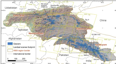
im-Figure 1.The study region in High Mountain Asia (HMA) covers four mountain ranges. Annotations denote locations of figures in the paper and points of orientation. International borders are tentative only as they are disputed in several regions.

proved significantly during recent years, during which sev-eral large-scale glacier inventories for HMA have been pub-lished – among others the Glacier Area Mapping for Dis-charge from the Asian Mountains (GAMDAM) inventory (Nuimura et al., 2015) and the second Chinese Glacier Inven-tory (CGI, Guo et al., 2015). Because the currently available version of GAMDAM only partially considered ice cover on steep slopes and the CGI only covered Chinese territory, a homogeneous basis for precise calculations covering all rele-vant catchments at the large scale is still missing. As both in-ventories have been combined for version 5.0 and transferred unchanged to version 6.0 of the Randolph Glacier Inventory (RGI) (Arendt et al., 2015; RGI Consortium, 2017), the re-lated regional-scale calculations using this version (e.g. Brun et al., 2017; Kraaijenbrink et al., 2017; Dehecq et al., 2015; Kääb et al., 2015) still suffer from uncertainties which stem from outlines of varying quality.

To overcome this situation, several regional-scale studies digitized glacier outlines themselves (e.g. Rankl and Braun, 2016; Minora et al., 2016) to have better control on data quality. But these again applied different criteria to delin-eate glacier extents and are thus not comparable to the ex-isting datasets, making change assessment difficult. On the other hand, the Karakoram and Pamir regions are character-ized by a high number of surge-type glaciers (Bhambri et al., 2017; Copland et al., 2011; Kotlyakov et al., 2008) with often strong geometric changes over a short period of time (Paul, 2015; Quincey et al., 2015). A precise inventory is

key to determine and maybe better understand such changes. Moreover, the large number of debris-covered glaciers in the region (Herreid et al., 2015; Minora et al., 2016) results in in-terpretation differences and is a large source of uncertainty.

The correct delineation of debris is also important for detecting very subtle past glacier changes (Scherler et al., 2011b) and to correctly model future glacier development (e.g. Kraaijenbrink et al., 2017; Shea et al., 2015), as surface mass balance of ice under a supraglacial debris layer is differ-ent from that of clean ice (Ragettli et al., 2015, 2016; Brock et al., 2010; Nicholson and Benn, 2006). The information on debris extent should thus be included in large-scale glacier inventories (Kraaijenbrink et al., 2017).

2 Study region

2.1 Location and glacier characteristics

The study area comprises a major share of the western part of HMA (Fig. 1). It stretches over∼300 000 km2and fully cov-ers the mountain ranges of (i) Pamir and its northern neigh-bour Pamir Alai in Uzbekistan, Turkmenistan, Kyrgyzstan, Tajikistan, Afghanistan and China and (ii) the Karakoram in Pakistan, India, and China.

The mountain ranges reach their highest elevations be-tween 5500 m (Pamir Alai) and more than 8600 m (Karako-ram, Hindu Kush), with K2 being the highest peak with 8611 m. Glaciers are found from ∼2300 m a.s.l. up to the highest peaks. The central Karakoram and inner Pamir are two of the most heavily glacierized mountain regions world-wide and include some extremely large glaciers such as Bal-toro, Siachen, and Fedchenko with sizes of about 810, 1094, and 573 km2, respectively. High peaks and deeply incised valleys create an extreme topographic relief that is also re-flected in the geometry of the glaciers, the majority of which are valley glaciers. In the Pamir, numerous cirques are also present, and hanging glaciers can be found at high eleva-tions in all regions. Larger, flat, high-altitude accumulation areas are rare and can only be found for some of the largest glaciers. Due to the steep terrain, most glaciers are partly fed by avalanches from the surrounding steep valley walls (Do-breva et al., 2017; Iturrizaga, 2011; Hewitt, 2011; Scherler et al., 2011a). This also causes an abundance of glaciers with partly or completely debris-covered tongues. Whereas debris cover makes glacier mapping difficult, the strong geometric changes in surging glaciers create additional challenges for glacier inventory compilation. Rock glaciers are present in all periglacial environments and are abundant also in our study region.

2.2 Climate

The climate of the study region can be subdivided into two major and independent regimes that define both the ther-mal and the moisture conditions. The Pamir and the ma-jor part of the Karakoram are predominantly influenced by westerly air flows throughout the year (e.g. Bookhagen and Burbank, 2010; Singh et al., 1995); towards the south-east the influence of the Indian summer monsoon (approx. June– September) becomes continuously stronger (e.g. Archer and Fowler, 2004). In general, outer western areas of the moun-tain ranges (Pamir Alai, western Pamir, Hindu Kush, south-eastern Karakoram) receive more precipitation, whereas fur-ther inland and to the east (eastern Pamir, central Karako-ram) the climate becomes drier and more continental (Lutz et al., 2014).

For most of the study region, the main share of pre-cipitation falls in winter and spring (Archer and Fowler, 2004; Bookhagen and Burbank, 2010). In regions

domi-nated by westerlies, winter precipitation is mostly advective, whereas convective precipitation plays an important role in drier regions and occurs predominantly in spring and summer (Böhner, 2006). In the eastern Pamir and also the central– eastern Karakoram, the precipitation peak is shifted towards spring, with important annual precipitation shares even in summer (Zech et al., 2005; Aizen et al., 2001, 1997). In monsoon-dominated regions (the border is roughly at 77◦E, Bookhagen and Burbank, 2010) a mixture of western dis-turbances and monsoon dominates in summer (Maussion et al., 2014; Böhner, 2006; Bookhagen and Burbank, 2010; Archer and Fowler, 2004). Little is known about tempera-ture and precipitation at the elevation of glaciers; stations in valley floors yield amounts between 70 and 300 mm yr−1 (Seong et al., 2009; Archer and Fowler, 2004). Precipitation amounts along the edge of mountain ranges and in high al-titudes are largely unknown, but can be substantially higher (“by a factor of ten”: Wake, 1989; Immerzeel et al., 2015), which is also suggested by snow station measurements show-ing snow accumulations of>1000 mm w.e. (millimetre wa-ter equivalent) around 4000 m in the Hunza basin (Winiger et al., 2005).

2.3 Glacier changes

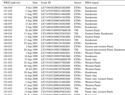
Table 1.List of Landsat scenes used to compile the inventory.

WRS2 path-row Date Scene ID Sensor HMA region

146-036 8 Oct 2000 LE71460362000282SGS00 ETM+ Karakoram

147-035 2 Aug 2002 LE71470352002214SGS00 ETM+ Karakoram

147-036 2 Aug 2002 LE71470362002214SGS00 ETM+ Karakoram

147-036 28 Aug 2000 LE71470362000241SGS00 ETM+ Karakoram

148-035 4 Sep 2000 LE71480352000248SGS00 ETM+ Karakoram

148-035 21 Jul 2001 LE71480352001202SGS00 ETM+ Karakoram

148-036 4 Sep 2000 LE71480362000248SGS00 ETM+ Karakoram

149-033 26 Jul 2009 LT51490332009207KHC00 TM Eastern Pamir

149-034 13 Aug 1998 LT51490341998225XXX01 TM Eastern Pamir, Karakoram

149-034 11 Sep 2000 LE71490342000255SGS00 ETM+ Eastern Pamir

149-035 13 Aug 1998 LT51490351998225XXX01 TM Karakoram

149-035 29 Aug 2001 LE71490352001241SGS00 ETM+ Karakoram

150-033 2 Sep 2000 LE71500332000246SGS01 ETM+ Eastern and western Pamir

150-034 20 Aug 1998 LT51500341998232BIK00 TM Eastern and western Pamir, Karakoram

150-034 2 Sep 2000 LE71500342000246SGS01 ETM+ Western Pamir

150-035 16 Sep 1999 LE71500351999259SGS00 ETM+ Karakoram

151-032 23 Sep 1999 LE71510321999266EDC00 ETM+ Pamir Alai

151-033 24 Aug 2000 LE71510332000237SGS00 ETM+ Western Pamir

151-034 30 Aug 2002 LE71510342002242SGS00 ETM+ Western Pamir

151-034 26 Jul 2001 LE71510342001207SGS00 ETM+ Western Pamir

151-035 30 Aug 2002 LE71510352002242SGS00 ETM+ Karakoram

152-032 16 Sep 2000 LE71520322000260SGS00 ETM+ Pamir Alai

152-033 16 Sep 2000 LE71520332000260SGS00 ETM+ Pamir Alai, western Pamir

152-034 2 Aug 2001 LE71520342001214SGS00 ETM+ Western Pamir

152-034 31 Aug 2000 LE71520342000244SGS00 ETM+ Western Pamir

153-032 15 Sep 2000 LT51530322000259XXX02 TM Pamir Alai

153-033 15 Sep 2000 LT51530332000259XXX02 TM Pamir Alai, western Pamir

154-033 29 Aug 2000 LE71540332000242EDC00 ETM+ Pamir Alai

and mass since the Little Ice Age (Holzer et al., 2016; Khro-mova et al., 2006; Shangguan et al., 2006).

3 Input data

As a mapping basis we have used six Landsat 5 TM and 22 Landsat 7 ETM+Level 1T scenes, with the latter offer-ing a 15 m panchromatic band for improved mappoffer-ing qual-ity (Table 1). Additionally, we have also used coherence images derived from the Advanced Land Observing Satel-lite 1 (ALOS-1) Phased Array type L-band Synthetic Aper-ture Radar 1 (PALSAR-1) scenes acquired around 2007 to aid in mapping the debris-covered glacier parts (Atwood et al., 2010; Frey et al., 2012) and the global digital elevation model (GDEM) version 2 from ASTER (hereafter referred to as GDEM2; United States Geological Survey, 2018a). The TM and ETM+scenes served as a basis for glacier map-ping while the coherence images were used for corrections of debris-covered glacier areas. Moreover, satellite images available in Google Earth served as a visual control for out-line detection, with data originating mainly from very high-resolution optical sensors such as QuickBird, Worldview,

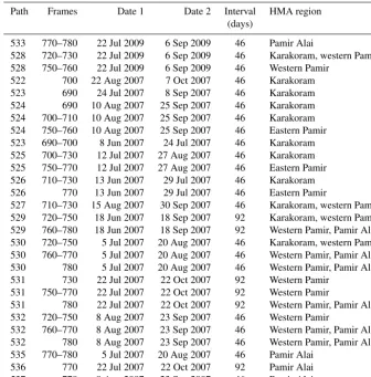
Pléiades 1A and 1B, and SPOT 6 and SPOT 7 (GoogleEarth 2017); unfortunately these were not available for all regions. Coherence images have been produced from ALOS-1 PALSAR-1 scenes usually separated by 46 days and acquired over summer (Table 2). The processing of the images takes into account a number of effects (e.g. sensor geometry, ra-diometric calibration, frequency interference) that influence the noise of the radar interferogram. The remaining decorre-lation can be ascribed to changes in landscape surface prop-erties, e.g. due to movement of landforms. More details on the processing line can be found in Frey et al. (2012).

par-Table 2.List of ALOS-1 PALSAR-1 scenes used to generate the coherence images.

Path Frames Date 1 Date 2 Interval HMA region

(days)

533 770–780 22 Jul 2009 6 Sep 2009 46 Pamir Alai

528 720–730 22 Jul 2009 6 Sep 2009 46 Karakoram, western Pamir

528 750–760 22 Jul 2009 6 Sep 2009 46 Western Pamir

522 700 22 Aug 2007 7 Oct 2007 46 Karakoram

523 690 24 Jul 2007 8 Sep 2007 46 Karakoram

524 690 10 Aug 2007 25 Sep 2007 46 Karakoram

524 700–710 10 Aug 2007 25 Sep 2007 46 Karakoram

524 750–760 10 Aug 2007 25 Sep 2007 46 Eastern Pamir

523 690–700 8 Jun 2007 24 Jul 2007 46 Karakoram

525 700–730 12 Jul 2007 27 Aug 2007 46 Karakoram

525 750–770 12 Jul 2007 27 Aug 2007 46 Eastern Pamir

526 710–730 13 Jun 2007 29 Jul 2007 46 Karakoram

526 770 13 Jun 2007 29 Jul 2007 46 Eastern Pamir

527 710–730 15 Aug 2007 30 Sep 2007 46 Karakoram, western Pamir

529 720–750 18 Jun 2007 18 Sep 2007 92 Karakoram, western Pamir

529 760–780 18 Jun 2007 18 Sep 2007 92 Western Pamir, Pamir Alai

530 720–750 5 Jul 2007 20 Aug 2007 46 Karakoram, western Pamir

530 760–770 5 Jul 2007 20 Aug 2007 46 Western Pamir, Pamir Alai

530 780 5 Jul 2007 20 Aug 2007 46 Western Pamir, Pamir Alai

531 730 22 Jul 2007 22 Oct 2007 92 Western Pamir

531 750–770 22 Jul 2007 22 Oct 2007 92 Western Pamir

531 780 22 Jul 2007 22 Oct 2007 92 Western Pamir, Pamir Alai

532 720–750 8 Aug 2007 23 Sep 2007 46 Western Pamir

532 760–770 8 Aug 2007 23 Sep 2007 46 Western Pamir, Pamir Alai

532 780 8 Aug 2007 23 Sep 2007 46 Western Pamir, Pamir Alai

535 770–780 5 Jul 2007 20 Aug 2007 46 Pamir Alai

536 770 22 Jul 2007 22 Oct 2007 92 Pamir Alai

537 770 8 Aug 2007 23 Sep 2007 46 Pamir Alai

ticular when using void-filled versions. A direct comparison (subtraction) of both DEMs as recommended by Frey and Paul (2012) confirmed these differences. We finally decided to work only with the GDEM2 as it had fewer data voids along mountain crests (important to derive correct drainage divides) and because it is spatially consistent; i.e. data voids over glaciers in the SRTM DEM did not have to be filled with some other DEM data (which is beneficial for deriving con-sistent topographic information and increases traceability). The vertical accuracy was found to be around 9 m (probably higher in steep terrain) and similar for both DEMs (Satgé et al., 2015). For consistency, the glacier separation and all sub-sequent topographic analysis of glacier elevation, slope, and aspect are thus based on the GDEM2.

4 Methods

4.1 Glacier mapping

We applied the well-established semi-automatic band ratio method (Paul et al., 2002) to classify glaciers (the clean-ice and snow part), taking advantage of the reflection contrast be-tween snow–ice and other land surfaces in the red and

short-wave infrared (SWIR) parts of the electromagnetic spectrum, corresponding to Landsat TM or ETM+bands 3 (red) and 5 (SWIR). An individual, scene-adjusted band ratio thresh-old between 1.5 and 3.5 is applied to separate glaciers and snow from other terrain and to compute a binary raster im-age, which is smoothed using a 3 by 3 majority filter and is then converted to a vector file for further editing.

Due to the spectral similarity of debris on and off glaciers, there is so far no method available to automatically map de-bris cover over a large set of glaciers using optical satellite imagery alone. Hence, several studies have tested combined approaches that generally include topographic information derived from a DEM and other data (Robson et al., 2016; Racoviteanu and Williams, 2012; Rastner et al., 2014; Bolch et al., 2007; Paul et al., 2004). However, all methods require time-consuming manual post-processing, and the quality of the results depends to some extent on the experience of the analyst.

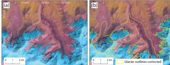
Figure 2.Mapping of heavily debris-covered tongues.(a)False-colour image overlaid by raw outlines.(b)PALSAR-1 coherence images overlaid by raw (yellow) and corrected (red) outlines. The decorrelated image areas are shown in black.

Figure 3.Elongated rock glaciers that are (almost) connected to the active glacier tongue are hard to distinguish.(a)False-colour Landsat image overlaid by raw outlines. (b)PALSAR-1 coherence images are fuzzy and potentially misleading in this case.(c)High-resolution imagery is decisive for a correct decision, because rock glaciers can be visually distinguished from the glacier tongue.

mapping in Alaska (Atwood et al., 2010) or as supportive means for correcting automatically derived glacier outlines in the western Himalaya by Frey et al. (2012). The coher-ence images were primarily used to detect the existcoher-ence of debris-covered glacier tongues, while the exact positions of the glacier margin and terminus were detected using the opti-cal Landsat image. The data are combined to account for the time difference of up to 9 years between coherence and Land-sat images. Non-surging debris-covered glaciers commonly change little during such periods (Scherler et al., 2011b), es-pecially in this region (e.g. Baltoro glacier has been stable for at least 25 years) (Paul, 2015).

The elevation of a glacier can be described by different el-evation parameters. One that is well suited for a comparison between different glacier types and sizes as well as an indi-cation for climatic differences is the median elevation, which

is indicative of the equilibrium line altitude (ELA) at a bal-anced mass budget (Braithwaite and Raper, 2009) and similar to the midpoint elevation (Raper and Braithwaite, 2009), that has been used in several studies to characterize glaciers (e.g. Haeberli and Hoelzle, 1995) and climatic conditions, primar-ily precipitation amounts (e.g. Sakai et al., 2015; Bolch et al., 2013).

4.2 Mapping challenges and solutions

Figure 4.Extensive moraines and large areas of debris can be found on dead ice and active glaciers.

Debris cover.The main reason for extensive debris cover on glaciers is steep/high topography with ice-free rock walls leading to rock falls and avalanches onto the glacier sur-face (e.g. Herreid et al., 2015; Scherler et al., 2011a; Paul et al., 2004). Apart from the central Karakoram, most re-gions exhibit glacier recession, which is another factor for increasing debris coverage on the glacier surface (Rowan et al., 2015; Kirkbride and Deline, 2013).

The debris-covered glacier area in this study was mapped manually by editing the automatically derived clean-ice out-lines. Key difficulties in identifying these regions are the small solar incidence angle at these latitudes (reducing topo-graphic contrast in the terminus region), unclear boundaries between supra-glacial debris and moraines or rock glaciers, and debris in shadow (e.g. Bishop et al., 2014). Heavily debris-covered glacier tongues are often in contact with lat-eral or frontal moraines (Figs. 2, 3, and 4) and their compo-sition is very similar, leading to similar spectral properties and the need of applying other measures for identification. Whereas human recognition has the ability to trace very sub-tle features for identification of debris on glaciers, the 30 m spatial resolution of Landsat images is often too coarse for a clear assignment.

In this study we mostly relied on the ALOS-1 PALSAR-1 coherence images for identifying the margins of debris-covered glaciers (Fig. 2). Their usability decreases with de-creasing glacier size as well as when the images become “fuzzy” and glacier margins less clear; in high-alpine terrain this could happen, as also glacier-free terrain can change: permafrost landforms such as rock glaciers, talus ramparts, and moraines complicate the proper identification of glaciers (Figs. 2, 3, and 4). In such cases we also used the very high-resolution imagery available in Google Earth and simi-lar tools for identification. Furthermore, multi-temporal data aided in terminus identification by either providing better contrast or by using them in animations (Paul, 2015). In some cases it was also possible to consider glaciological relations for a first approximation of glacier extent. For example, a tiny accumulation area would likely not support a large glacier tongue (and vice versa).

In contrast to glaciers – massive bodies of ice originating from continuous snow accumulation – rock glaciers probably have a different genesis: they develop in a permafrost envi-ronment either from ice-cored moraines or on talus slopes that provide constant debris input, and they commonly have a higher debris content than glaciers (Berthling, 2011; Hae-berli et al., 2006; Barsch, 1996). Especially towards the cold–dry regions of central Asia, rock glaciers of both types are increasingly abundant (Bolch and Gorbunov, 2014; Gor-bunov and Titkov, 1989). In particular, moraine-derived rock glaciers challenge the analyst as there is often a continu-ous transition between the glacier and the rock glacier, mak-ing it hard to define a divide (cf. Monnier and Kinnard, 2015). A well-developed rock glacier can in principle be distinguished from a debris-covered glacier by characteris-tic surface patterns such as the arc-shaped transverse ridge and furrow structure instead of the longitudinal debris stria-tions and supra-glacial ponds found on most debris-covered glaciers (Bishop et al., 2014; Bodin et al., 2010). However, identifying such differences using remotely sensed imagery requires a spatial resolution better than 15 m (Paul et al., 2003) and might not work at all when rock glaciers are not well developed. We separated debris-covered glaciers from rock glaciers based on interpreting the above data sources (Google Earth, coherence images) and their known morpho-logical characteristics. In the cases where no clear boundary could be found, we followed a more conservative interpreta-tion that might have resulted in a potential underestimainterpreta-tion of the debris-covered glacier area.

Figure 5.Glacier detection in shadow with the supporting input of high-resolution Google Earth images.

some parts of the northern–central Karakoram, potentially re-sulting in related higher area uncertainties for the accumula-tion areas of the glaciers. Our strategy to reduce the impact of wrongly mapped seasonal snow was threefold: we applied a size filter of 0.02 km2to remove the smallest snow patches; snow attached to glaciers was manually removed after visual inspection, and in some regions a different scene (with less snow but possibly more clouds) was chosen to improve re-sults (see Table 1). Despite these measures, we assume that glacier area in this inventory is likely overestimated due to the inclusion of seasonal snow.

Shadow. Cast shadows from mountains decrease reflec-tion values, partly down to near-zero. This results in con-siderable noise in this region for a band ratio using a red (or near infrared) band. As TM band 1 (blue) is strongly influ-enced by atmospheric scattering, ice and snow in shadow are much more visible and can be distinguished using an addi-tional threshold (e.g. Paul and Kääb, 2005). Although the shadow problem is less pronounced in lower latitudes due to the higher solar elevation angle, it is still a problem in the study region due to the high and steep terrain. We have used the additional blue band to map glaciers in shadow automat-ically or applied manual corrections on contrast-enhanced true-colour composites in case the automated refinement was not successful. We also analysed scenes from a different date or another sensor (including very high-resolution imagery as available in Google Earth and similar tools) to reveal if glaciers are possibly present (Fig. 5). However, this is time-consuming and in some regions images are not available or do not meet the criteria for glacier identification (e.g. due to snow cover). In the cases where glaciers in shadow could not be identified, a related underestimation of glacier area results. Cloud coverage. Cloud-free scenes were available for most of the study region. In the few cases when cloud cover prevented glacier mapping, the problem was solved multi-temporally by using additional scenes from years close to the year 2000 (Paul et al., 2017). In some regions, scenes with high cloud coverage and possible precipitation events were followed by scenes with extensive snow coverage, so that we had to use scenes from other years. The entire study region is thus a mosaic of many individual scenes (see Table 1).

Figure 6.Debris cover classification in the Kongur Shan in the east-ern Pamir.

4.3 Calculating the debris-covered area share of glaciers

For calculating the area share of debris cover, we decided to consider only the ablation areas of glaciers (i.e. the region below their median elevation), because debris deposited in the accumulation area should emerge on the glacier surface only below the ELA (Braithwaite and Raper, 2009; Braith-waite and Müller, 1980). We distinguished the debris cover from snow and ice surfaces by applying a constant thresh-old of 2.0 to all band ratio images from Landsat TM bands 3 and 5 (red and SWIR) and subtracted the resulting clean-ice glacier map from the corrected glacier map. The threshold was found empirically with satisfying results for all scenes from TM and ETM+ sensors. Changing the threshold by ±0.2 changed the result by less than the mapping uncertain-ties (∼5 % for debris-covered areas, see Sect. 6).

4.4 Glacier definition and separation using drainage divides

in-cludes “all tributaries and connected feeders that contribute ice to the main glacier, plus all debris-covered parts of it”. For the sake of consistency with earlier datasets and the GLIMS definition, surge-type tributaries were not separated from the main glacier tongue, even if they contribute only during an active surge phase. The preparation of a dataset where these short-term tributaries are properly separated is worthwhile but a considerable extra effort. Stagnant ice masses (e.g. from a former surge) that were still connected to the glacier tongue were mapped as part of the glacier. In cases where the active glacier has clearly receded away from the stagnant “dead” ice (e.g. after a surge phase), only the active glacier was mapped. In contrast to this definition, the surging Bivachny glacier tongue was separated from Fedchenko glacier in the confluence region although one can argue that Bivachny is a connected feeder (see Fig. 6 in Wendt et al., 2017). A size fil-ter of 0.02 km2was applied to remove small seasonal snow-fields and remaining noise. Automatically classified poly-gons larger than this are considered as glaciers in this in-ventory, but this does not mean that all seasonal or perennial snowfields have been excluded, nor that some of the mapped glaciers are in fact perennial snow.

Glacier complexes – at least two glaciers connected in their accumulation areas – can be split into single glaciers using drainage divides derived from a DEM. This is per-formed in two steps. Firstly, raw drainage basins are cal-culated by watershed analysis using a flow direction grid derived from a sink-filled DEM. Afterwards, overlying raw basins are merged to one basin polygon per glacier consid-ering pour points and a buffer (Falaschi et al., 2017; Kien-holz et al., 2013; Bolch et al., 2010). This approach proved to be robust even for the large regions of the Karakoram and Pamir as in general glaciers are divided by very steep moun-tain crests. Secondly, manual corrections were performed, which took about 90 % of the total processing time. Gross er-rors were improved using a colour-coded flow direction grid in the background, a hillshade, the original Landsat scenes, and sometimes oblique views in Google Earth. We manu-ally assigned the same ID to separated glacier polygons that were obviously linked by mass transport (e.g. regenerated glaciers).

4.5 Uncertainty estimation

Since there is no ground truth or reference data for any larger set of glaciers in the study region, we calculated uncertain-ties for the relevant input data rather than accuracy (Paul et al., 2017).

Glacier mapping uncertainties originate from the cover-age of glaciers by seasonal snow and/or debris, shadow, and clouds. These need to be corrected manually (on-screen dig-itizing) by a well-trained analyst. According to the litera-ture, the uncertainty of automatically and manually digitized glacier outlines (clean ice only) ranges between 2 % and 5 % and is dependent on glacier size (Paul et al., 2013, 2011;

Andreassen et al., 2008; Bolch and Kamp, 2006). Paul et al. (2013) estimated uncertainties using a sample of manu-ally and automaticmanu-ally digitized glaciers from a number of experts and found a mean standard deviation of∼5 %. Other studies (Bolch et al., 2010; Granshaw and Fountain, 2006) have used a buffer-based estimate, where the final uncer-tainty depends on the pixel size of the input image. The study by Paul et al. (2017) suggested a tiered system of uncer-tainty assessment related to workload. We used three of the methods: (1) fixed uncertainty values applied to all glaciers, (2) the buffer method with different buffer sizes for clean and debris-covered glacier parts, and (3) independent multi-ple digitization of outlines by all analysts for three difficult debris-covered glaciers.

For (1), we applied an uncertainty of±2 % for the clean ice and ±5 % for the debris-covered ice. This is an up-per boundary estimate, because it does not account for the overlapping area of the two surface types. For the buffer method (2) we applied an uncertainty of ±1/2 pixel for clean-ice parts and±1 pixel for debris-covered parts. This also provides an upper-bound estimate and we use the stan-dard deviation of the uncertainty distribution for the esti-mate, as a normal distribution can be assumed for this type of mapping error. It is applied to glacier complexes exclud-ing overlappexclud-ing areas as well as the border of clean and debris-covered ice of the same glacier. Due to the abun-dant debris-covered glaciers in the study region, we also per-formed method (3) to obtain a more realistic uncertainty es-timate for the analysts participating in the outline correc-tion. They manually corrected the outlines of three exam-ple glaciers from different regions three times (Glacier 1: 38◦_34.40_{N, 72}◦_12.80_{E; Glacier 2: 39}◦_38.80_{N, 69}◦_41.90_E; Glacier 3: 36◦_0.30_{N, 75}◦_14.60_{E), with differing additional} information being considered (e.g. coherence images and Google Earth imagery). The glaciers are of different size and contain a substantial debris-covered part; they also fea-ture difficulties of moraines, glacier confluences, and cast shadow.

As not all satellite scenes used to compile the inventory are from the same year, there is a certain temporal uncer-tainty introduced. However, glacier changes within the± 2-year difference to the target 2-year 2000 are likely within the uncertainty of the glacier outlines and should thus not mat-ter. The actual date information is given for each glacier in the attribute table.

5 Results

5.1 Basic statistics

Table 3.The upper table shows the basic inventory statistics for all glaciers, with the lower table only showing the basic inventory statistics for glaciers larger than 5 km2.

Glacier area Uncertainty Mean of

(km2) (km2)

glacier area median elev. slope max. elev. min elev. no. of

(km2) (m) (◦) (m) (m) glaciers

All glaciers

All 35519.7 ±1948 1.27 4993 26.4 5251 4739 27 877

Pamir Alai 2078.5 ±114 0.57 4147 25.1 4359 3962 3655

Pamir west 9469.4 ±519 0.85 4871 25.5 5105 4654 11 098

Pamir east 2277.2 ±125 0.98 5050 26.4 5305 4801 2326

Karakoram 21694.6 ±1190 2.01 5392 27.7 5693 5076 10 798

Glaciers≥5 km2

All 22299.9 ±1223 22.5 5173 22.6 6135 4250 990

Pamir Alai 673.1 ±37 12.9 4111 19.5 5024 3379 52

Pamir west 4754.5 ±261 17.3 4882 21.7 5806 4107 275

Pamir east 1089.7 ±60 15.1 5196 25 6342 4204 72

Karakoram 15782.6 ±866 26.7 5399 22.9 6362 4399 591

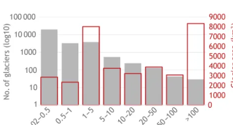
Figure 7.Histogram of all glaciers by number. Please note the log-arithmic scale of the leftyaxis.

compiled (e.g. Kienholz et al., 2015; Guo et al., 2015; Pfef-fer et al., 2014; Le Bris et al., 2011; Bolch et al., 2010), the histogram is strongly skewed towards small glaciers (Fig. 7). Only 3.5 % (985) of all glaciers are larger than 5 km2, and most of them are located in the Karakoram. In total, they cover over 60 % of the glacierized area. On the other hand, 83 % (23 048) of all glaciers are smaller than 1 km2but cover only∼15 % of the total area. The mean glacier size is 1.29 km2, with large differences between the regions: from 0.57 km2 in the Pamir Alai to 2.07 km2 in the Karakoram (Table 3). The average median elevation is 4978 and 5169 m for all glaciers and glaciers larger than 5 km2, respectively, and differs by only a few metres from the mean elevation.

5.2 Extremes

In the Pamir Alai, the largest glacier is Zeravshan glacier, with an area of 106.3±6.7 km2, which is 3 times larger than the second largest. Zeravshan glacier stretches over 2600 m from 2800 to 5400 m, close to the highest elevations in the Pamir Alai range. The largest elevation range is covered by Tandykul glacier (39◦270N, 71◦80E) 50 km further east, with almost 3000 m (2450–5400 m). Its heavily debris-covered tongue lies in a deep valley that is well shielded from the south. Overall, only a few larger valley glaciers (19 larger than 10 km2) have several large tributaries.

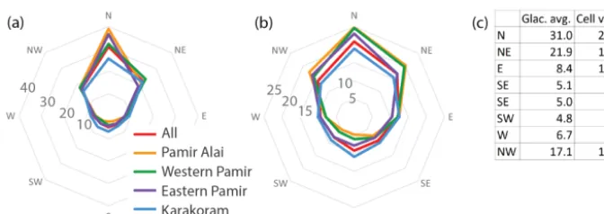
Figure 8.Glacier orientation of the different HMA regions.(a)shows the values based on average glacier aspect;(b)is based on the 30 m raster cells. Lower elevations tend to have a higher share of the north-facing glacier area. The respective numbers of “All” are given in the table(c).

Figure 9. Slope per glacier regions and surface type (avg. slp.: average slope of glacierized area; avg. slp. acc.: average slope in the accumulation area; avg. slp. abl.: average slope in the ablation area; avg. slp. deb.: average slope in the debris-covered area).

(70.65◦E/38.99◦N) in the Petra Pervogo Range, reaching down to below 2400 m.

The eastern Pamir region has 38 glaciers larger than 10 km2, evenly distributed over the individual mountain ranges. The largest glacier (109.4±6.9 km2) is Karayaylak glacier, draining the northern basin of the Kongur Shan. It starts at the top of Kongur Tagh, with the highest mountain in the Pamir at an elevation of 7680 m, and reaches down to 2819 m, spanning an elevation range of over 4800 m, which is by far the largest value in this region. One of its tributaries has reportedly surged in 2015 (Shangguan et al., 2016). The neighbouring Qimgan glacier starts at the same peak facing south-east and reaches down to 3160 m (almost 4500 m el-evation range). A smaller, east-facing glacier in the Oytagh glacier park reaches the same low elevation as Karayaylak glacier (2824 m).

Siachen glacier is the largest of its kind in the Karakoram. With an area of 1094.2±31.2 km2(including all of its ma-jor tributaries) it is by far the largest glacier in the study area, and with over 70 km in length Siachen and Fedchenko are the longest glaciers in the mid-latitudes. Two more glaciers have an area over 500 km2: Baltoro with 810±36.1 km2and Biafo with 560±23.8 km2. Both glaciers reach their lowest eleva-tions in the central part of the Hunza valley (around Gilgit),

with terminus elevations of around 2500 m and below (Hopar glacier: 2260 m). Two large glaciers reach elevation ranges of 5200 m (Batura and Baltoro), but also smaller glaciers like Shishper (45±4.1 km2), Passu (62.2±1.7 km2), and Raka-poshi (14.4±0.9 km2) stretch over an elevation range of 5000 m. Once again, many of these glaciers are of a surge type (e.g. Bhambri et al., 2017), and their minimum eleva-tions and area values after a surge might strongly differ from those at the end of a quiescent phase. The highest glacier-ized regions in the Karakoram are found around K2 (8611 m; Baltoro glacier) and Distaghil Sar (7885 m; Yazghil glacier, Hispar glacier).

5.3 Glacier aspect analysis

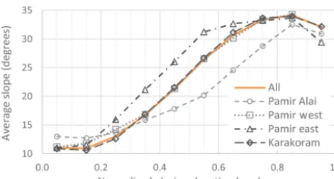
re-Figure 10.Glacier slope along 10 glacier elevation sections. The glaciers were normalized for elevation to compare high- and low-elevation glaciers.

gions (mean: 56.5 %±5.7 %, Fig. 8b), while the south and south-west host the smallest share of glacierized area.

In contrast to other regions, we found no correlation be-tween median elevation and aspect.

5.4 Glacier slope analysis

The mean slope of all glaciers is 26.4◦. It decreases to 22.6◦ for glaciers larger than 5 km2; hence, mean slope is size de-pendent. The decrease in mean slope between the sample of all glaciers and glaciers larger than 5 km2is relatively large for Pamir Alai (−5.6◦_{) and very small for the eastern Pamir} (−1.4◦_{). Mean slope varies between different parts of the} glacier, with the accumulation area being the steepest section and the debris-covered areas being far flatter in all regions (Fig. 9).

To determine whether glaciers constantly get steeper from the terminus to the upper reaches of the accumulation area, we normalized the elevation distribution of all glaciers such that each glacier covered the value range from 0 to 1 from the terminus to the upper end, divided into sections of 0.1. The result clearly reveals a mean slope of about 12◦in the lower parts and a constant increase to over 30◦at the highest elevations of each glacier (Fig. 10). The uppermost band is again somewhat flatter, possibly due to the transition of slope direction at crests. The pattern is similar in all regions, but the slope increase along the glacier is higher than average in the eastern Pamir and lower than average in the Pamir Alai.

5.5 Glacier elevation analysis

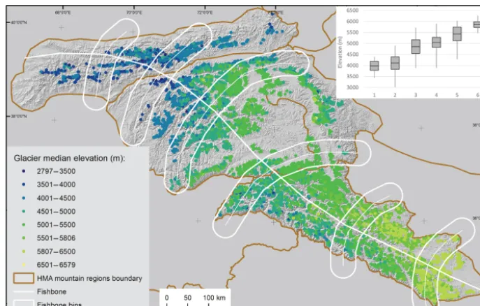
The median elevation of glaciers larger than 2 km2 ranges from 2800 to over 6500 m. There is a statistically significant correlation (p <0.001) between median elevation and lati-tude (r2=0.48) and longitude (r2=0.66), which appears as a rise of median elevation from the north-west towards the south-east across the study region (Fig. 11).

This rise becomes even clearer when looking at separated areas along a “fishbone” transverse profile of our study

re-gion (inset). The average values of each segment reveal a rise in median elevation from 3980 m (bin 1) to 5860 m (bin 6), with an average trend of 1.9 m km−1_{along the profile.}

5.6 Hypsography

Plotting the glacier hypsography of the different HMA re-gions (Fig. 12a) reveals a number of further differences among the regions. Most apparent is the difference in eleva-tion: the median elevation extends from 4141 m (Pamir Alai) to 5419 m (Karakoram), with the western Pamir (4941 m) and eastern Pamir (5119 m) in between the two. Most of the glacierized area is located in the Karakoram (60 %) where the ice is distributed over a large elevation range (Fig. 12b). In contrast, in the Pamir Alai most of the glacier area is situated closely around the median elevation. The large glaciers in the Karakoram reach far down and occupy large areas in lower elevations, further away from the median elevation than in other regions. The eastern Pamir shows a similar drop in the area share of higher elevations, but the curve flattens in ele-vations over 1000 m above the median elevation. This is re-lated to the shape of topography that is dominated by distinct mountain ranges with large areas above 6500 m (Kongur, Muztag Ata, Kingata Shan). When analysing the hypsog-raphy of glaciers with over 10 % debris-covered area com-pared to the rest of the sample, the insulation effect becomes visible, with debris-covered glaciers occupying considerably more area at lower elevations (Fig. 12c).

5.7 Debris cover

Figure 11.Glacier median elevation over the study area of glaciers larger than 0.5 km2. The inset shows median elevation, standard devia-tions, and minimum and maximum elevations per bin.

Generally, there is no relation between the mean slope of a glacier and the area share of its debris cover. However, the mean slope of the debris-covered part of the glaciers is 16.6◦ (±5.5), whereas the mean slope of these glaciers is 26.1◦ (±3.2). This was expected since the debris cover is usu-ally situated at the flatter glacier tongues (Paul et al., 2004). Looking at the ablation area of all glaciers, the mean slope is 25.0◦(±4.2). The ablation areas of more strongly covered glaciers are somewhat flatter: glaciers with a debris-covered area of≥10 % on average have a steepness of 22.7◦ (±4.0); in contrast, glaciers with less than 5 % debris cover have a mean slope of 25.7◦(±4.1).

6 Uncertainties and the multiple digitizing experiment

By applying previously assumed area uncertainties (±2.5 % for clean ice, ±5 % for debris-covered ice) to the mapped glacier area, the derived total glacier area is 35 520± 1955 km2. With the buffer method (clean ice±1/2, debris-covered ice±1 pixel) we obtain a similar uncertainty of ±1948 km2. Both methods are applied to glacier complexes to avoid double counting of overlapping areas of adjacent glaciers. Finally, the multiple digitization experiment re-sulted in a±13 % standard deviation (averaged over all ex-periments). This value appears high, but it reflects the map-ping reality in challenging situations with debris-covered glacier tongues. For two of the three test glaciers, the differ-ence between the largest and the smallest area mapped was less than 5 % of the mean glacier area. The third example is a small (∼2.9 km2) and steep glacier with a high share of

its area hidden in shadow, a large and barely visible debris-covered part and adjacent rock glaciers (see Fig. S2 in the Supplement). Here, the respective uncertainty is±33 %. Tak-ing this as a worst-case scenario, only few such cases exist in a larger inventory and the high uncertainty has little impact on the overall uncertainty.

Paul et al. (2013, 2015) showed that analyst interpreta-tions for debris-covered glaciers and glacier parts in shadow can differ by up to 50 %. Our experiment showed that, if the glacier is affected by both shadow and debris cover and is ad-ditionally small, the differences can be even higher with up to 70 %. The experiment also confirmed that area differences mainly depend on the interpretation of the debris-covered parts. Thereby, using coherence images improved the ana-lyst’s interpretation. Although the overall effect was small (on average∼1 %), it reduced the dispersion of the analyst’s interpretations considerably (see Fig. 14). The different tim-ing of Landsat (2000) and ALOS-1 PALSAR-1 (2007–2009) imagery had only a small impact, as geometric changes dur-ing these 7 years were small. The use of Google Earth im-agery did not lead to notable outline modifications as they either had low quality (resolution, snow cover) or provided a mere confirmation of the existing interpretation from Landsat and coherence images. We conclude that the area uncertainty of the debris-covered parts of a glacier is of the order of 10 % to 20 %. However, at least one third of this uncertainty can be disregarded due to direct contact to clean-ice glacier parts (see Fig. 13).

Figure 12.Glacier hypsography of the different regions(a), normalized by the respective median elevation(b). Dashed lines represent the 25 % and 75 % area elevations.(c)Hypsography comparison of more and less debris-covered glaciers.

Figure 13.Debris cover on glaciers in the central Karakoram.

of the debris-covered area, which is smaller than the un-certainty from the manual correction of the debris-covered glacier parts.

All uncertainty values have to be seen from the perspective of methodological uncertainties, e.g. the inclusion of possi-ble snowfields at high elevations, which can easily increase the area of a small glacier by 50 % or more. With this in mind, the uncertainties presented above are in general much smaller

and are more of an academic nature. As the uncertainties from the expert round robin are close to those from the buffer method, we use the uncertainty derived by the buffer method as the uncertainties assigned to our results, knowing that they are on the conservative side.

Figure 14.Results of the expert round robin, example Glacier 2.(a)shows mapping results solely based on the satellite image, whereas (b) shows mapping results after manual corrections using the additional source of coherence images and Google Earth high-resolution imagery.

Figure 15.Comparison example of the three inventories.

We think that excluding steep headwalls leads to an incom-plete inventory and that the inclusion of rock outcrops in the CGI constitutes a commission error that needs to be corrected for some applications. Overall, the differing interpretation of debris-covered glacier parts and seasonal snow is seemingly the main source of differences in glacier extents for the same region when mapped by different analysts.

7 Discussion

When compiling a large-scale glacier inventory, it is essen-tial to have homogeneous quality of the input data used, at best also in a temporal sense, to ensure high credibility of the resulting outlines and topographic parameters as well as low

uncertainties of the glacierized area. This can be achieved by using globally consistent datasets such as the Landsat im-ages and the GDEM2. However, the latter does not fulfil the criterion of temporal consistency and future work might overcome this issue. There are strategies like DEM fusion to improve DEM quality in regions of very steep terrain or low-contrast glacier surfaces (e.g. Shean et al., 2016; Lee et al., 2015; Tran et al., 2014 and references therein), but the impact of such quality issues is difficult to assess without ac-curately geo-referenced high-resolution reference data (Kääb et al., 2016; Frey and Paul, 2012). With the semi-automated processing line applied here and the few experts involved in the manual corrections, we assume a homogeneous quality of the glacier outlines throughout the study area has been achieved. However, our glacier extents are likely on the con-servative side for debris-covered ablation areas, leading to an underestimation of glacier area, whereas the included peren-nial ice and snowfields in steep terrain at high elevations are more generous than in other interpretations.

A major prerequisite for all methods is the use of glacier out-lines that are well adjusted for debris cover. Glacier retreat was found to correlate with an increase in supraglacial debris cover (e.g. Stokes et al., 2007) and, hence, multi-temporal mapping of debris extent should be applied. As extensive debris cover affects glacier melt and geometry (e.g. Ander-son and AnderAnder-son, 2016), we recommend including it in the published glacier inventories (GLIMS, RGI), by (a) adding the debris mask as a polygon and (b) including debris cover share in the attribute table. Our results show a total of∼10 % debris-covered area, with many of the larger glaciers reach-ing 20 % or more. These numbers complement and confirm existing estimates in HMA that are based on smaller sam-ples. Values reported from the central Karakoram are 20 % (Minora et al., 2016) and∼21 % (Herreid et al., 2015), Frey et al. (2012) calculated 16 % for the western Himalaya, and for the entire Himalaya a ∼10 % coverage was calculated (Kraaijenbrink et al., 2017; Bolch et al., 2012).

Comparing the freely available results by Kraaijenbrink et al. (2017) to our results, the total difference is <1.5 % of the total debris-covered area (3365 km2vs. 3409 km2), a value well below the uncertainty of these areas. However, the differences vary from one region to another, from−18.4 % in the Pamir west to 5.7 % in the Karakoram.

The pattern of glacier median elevations found in our study reflects combinations of climatic and topographic aspects. A similar west–east and north–south gradient was also found in the study by Sakai et al. (2015), who determined median elevations from a glacier inventory (GAMDAM, Nuimura et al., 2015) for all of HMA. Whereas the latitudinal extent of 7◦decreases air temperatures and thus median elevations to-wards the north, the precipitation decrease from west to east due to leeward rain shadow effects increases median eleva-tions in the eastern Pamir and Karakoram. Approximating the balanced-budget ELA (ELA0) with the median elevation has been successfully applied in many mountain ranges and works well for different glacier types (Braithwaite and Raper, 2009). However, this concept likely does not apply to surge-type glaciers and glaciers that are mainly nourished by snow avalanches (Hewitt, 2011). For the latter as well as debris-covered glaciers, ELA0values are expected to be higher than those calculated here due to the additional accumulation and reduced ablation. This is supported by the fact that we find debris-covered areas also above the median elevation and by a finding from Braithwaite and Raper (2009), who mention possible accumulation-area ratio values below 0.5 for Hi-malayan glaciers.

We also performed a detailed analysis of uncertainties and analysed the most important sources contributing to uncer-tainty. It is, however, impossible to perform a rigorous cal-culation, as this would require a comparison with appropri-ate reference data. The uncertainties presented here are based on different methods and some of the values are higher than reported previously. This is mainly because of the high de-bris coverage and the large number of (very) small glaciers.

Under such challenging conditions, area differences among the analysts were as high as uncertainties due to the possible wrong consideration of seasonal snow. Hence, the total area of our inventory will likely be somewhat larger than other inventories for this region as these might have excluded the maybe just snow-covered steep regions at highest elevations. Once scenes without seasonal snow in these regions become available, glacier extents should be revisited and corrected as required.

8 Data availability

The dataset is downloadable at

https://doi.org/10.1594/PANGAEA.894707 (Mölg et al., 2018).

9 Conclusion

We derived a new glacier inventory for a substantial part of western High Mountain Asia (Karakoram and Pamir) and have presented in detail the derived characteristics of the glaciers in this region. Special emphasis was given to the de-scription of mapping challenges for debris-covered glaciers (and distinguishing them from rock glaciers), seasonal snow, and shadow, along with the selected solutions. In the ab-sence of appropriate reference datasets, we instead applied various methods for uncertainty assessment and compared our outlines to other existing inventories covering the same region. As an extension to already existing datasets we in-cluded outlines and percentages of the debris-covered area for each glacier.

We mapped 27 437 glaciers covering 35 287±1209 km2, with about 10 % of the area being debris covered. The ASTER GDEM2 was found to be superior to the SRTM DEM (1 arcsec) in deriving drainage divides and topographic information for each glacier as the latter suffered from too many (wrongly interpolated) data voids in this region. The application of a constant band ratio threshold to derive clean-ice areas for all scenes to create the debris cover maps was found to be of sufficient quality. Uncertainties derived from three different methods were all in good agreement (3.4 %) but the multiple-digitizing experiment also revealed larger deviations among the analysts under challenging conditions (debris, shadow, small glacier). However, the availability of coherence images improved the quality and consistency of the manual corrections for debris-covered glaciers consider-ably.

one on longitude and latitude (higher towards the drier north and east), indicating a close relation to precipitation amounts. Glacier hypsometry reveals a peak distribution that is high-est (∼5700 m) in the Karakoram, similar but 700 m lower in the eastern and western Pamir, and lowest in Pamir Alai (∼4200 m). Glaciers in the Karakoram have a comparably higher area share at the lowest elevations and glaciers larger than 5 km2 or debris-covered glaciers are flatter (22.6 and 16.6◦, respectively) than on average (26.4◦). By location, glaciers are especially flat (<15◦) in their lowest third and progressively steeper (>30◦) in the uppermost third, indi-cating the dominance of large valley glaciers with very flat tongues and steep head walls. Both glacier outlines and the separate outlines of the debris-covered parts will be freely available from the GLIMS database to facilitate applications such as distributed mass balance modelling and albedo calcu-lation; debris-thickness calcucalcu-lation; determination of run-off (with a melt reduction under debris-covered areas); and fu-ture geometric evolution, sediment transport, and mountain erosion rates, to name a few.

Supplement. The supplement related to this article is available online at: https://doi.org/10.5194/essd-10-1807-2018-supplement.

Author contributions. NM, FP, TB, and PR designed the study. NM and FP wrote the manuscript. NM, PR, TB, and FP generated and edited glacier outlines and basins. TS produced the coherence images. NM extracted debris cover and performed all analysis. All authors contributed to the final form of the manuscript.

Competing interests. The authors declare that they have no con-flict of interest.

Acknowledgements. We thank J. Graham Cogley and an anonymous reviewer as well as the journal editor for their thor-ough reviews and constructive comments that helped improve the clarity of the paper. We acknowledge funding from the ESA projects Glaciers-cci (4000109873/14/I-NB) and Dragon 4 (4000121469/17/I-NB) as well as the Copernicus Climate Change Service (C3S) that is implemented by ECMWF on behalf of the European Commission. The manual digitizing experiment was performed by the authors with additional contributions by Holger Frey and Raymond Le Bris.

Edited by: Reinhard Drews

Reviewed by: J. Graham Cogley and one anonymous referee

References

Aizen, E. M., Aizen, V. B., Melack, J. M., Nakamura, T., and Ohta, T.: Precipitation and atmospheric circulation

pat-terns at mid-latitudes of Asia, Int. J. Climatol., 21, 535–556, https://doi.org/10.1002/joc.626, 2001.

Aizen, V. B., Aizen, E. M., Melack, J. M., and Dozier, J.: Climatic and Hydrologic Changes in the Tien Shan, Central Asia, J. Cli-mate, 10, 1393–1404, 1997.

Anderson, L. S. and Anderson, R. S.: Modeling debris-covered glaciers: response to steady debris deposition, The Cryosphere, 10, 1105–1124, https://doi.org/10.5194/tc-10-1105-2016, 2016. Andreassen, L. M., Paul, F., Kääb, A., and Hausberg, J. E.:

Landsat-derived glacier inventory for Jotunheimen, Norway, and deduced glacier changes since the 1930s, The Cryosphere, 2, 131–145, https://doi.org/10.5194/tc-2-131-2008, 2008.

Archer, D. R. and Fowler, H. J.: Spatial and temporal variations in precipitation in the Upper Indus Basin, global teleconnections and hydrological implications, Hydrol. Earth Syst. Sci., 8, 47–61, https://doi.org/10.5194/hess-8-47-2004, 2004.

Arendt, A., Bliss, A., Bolch, T., Cogley, J. G., Gardner, A. S., Ha-gen, J.-O., Hock, R., Huss, M., Kaser, G., Kienholz, C., Pfef-fer, W. T., Moholdt, G., Paul, F., Radi´c, V., Andreassen, L. M., Bajracharya, S., Barrand, N. E., Beedle, M., Berthier, E., Bham-bri, R., Brown, I., Burgess, E. W., Burgess, D., Cawkwell, F., Chinn, T., Copland, L., Davies, B., Angelis, H. de, Dolgova, E., Earl, L., Filbert, K., Forester, R., Fountain, A. G., Frey, H., Giffen, B., Glasser, N. F., Guo, W., Gurney, S. D., Hagg, W., Hall, D., Haritashya, U. K., Hartmann, G., Helm, C., Herreid, S., Howat, I., Kapustin, G., Khromova, T. E., König, M., Kohler, J., Kriegel, D., Kutuzov, S., Lavrentiev, I., Le Bris, R., Liu, S., Lund, J., Manley, W., Marti, R., Mayer, C., Miles, E. S., Li, X., Menounos, B., Mercer, A., Mölg, N., Mool, P., Nosenko, G., Ne-grete, A., Nuimura, T., Nuth, C., Pettersson, R., Racoviteanu, A., Ranzi, R., Rastner, P., Rau, F., Raup, B., Rich, J., Rott, H., Sakai, A., Schneider, C., Seliverstov, Y., Sharp, M. J., Sigurðsson, O., Stokes, C. R., Way, R. G., Wheate, R., Winsvold, S., Wolken, G., Wyatt, F., and Zheltihyna, N.: Randolph Glacier Inventory – A Dataset of Global Glacier Outlines: Version 5.0: GLIMS Tech-nical Report, Global Land Ice Measurement from Space, Col-orado, USA, Digital Media, https://doi.org/10.7265/N5-RGI-50 (last access: 13 March 2018), 2015.

Atwood, D. K., Meyer, F., and Arendt, A.: Using L-band SAR co-herence to delineate glacier extent, Can. J. Remote Sens., 36, S186–S195, https://doi.org/10.5589/m10-014, 2010.

Bajracharya, S. R., Maharjan, S. B., Shrestha, F., Guo, W., Liu, S., Immerzeel, W., and Shrestha, B.: The glaciers of the Hindu Kush Himalayas: Current status and observed changes from the 1980s to 2010, Int. J. Water Resour. D., 31, 161–173, https://doi.org/10.1080/07900627.2015.1005731, 2015. Barsch, D.: Rockglaciers: Indicators for the Present and Former

Geoecology in High Mountain Environments, in: Springer Se-ries in Physical Environment, Springer Berlin Heidelberg, Berlin, Heidelberg, 16, 331 pp., 1996.

Berthling, I.: Beyond confusion: Rock glaciers as

cryo-conditioned landforms, Geomorphology, 131, 98–106,

https://doi.org/10.1016/j.geomorph.2011.05.002, 2011. Bhambri, R., Bolch, T., Kawishwar, P., Dobhal, D. P., Srivastava,

D., and Pratap, B.: Heterogeneity in glacier response in the upper Shyok valley, northeast Karakoram, The Cryosphere, 7, 1385– 1398, https://doi.org/10.5194/tc-7-1385-2013, 2013.

Reports, 7, 15391, https://doi.org/10.1038/s41598-017-15473-8, 2017.

Bishop, M. P., Shroder, J. F., Ali, G., Bush, A. B. G., Haritashya, U. K., Roohi, R., Sarikaya, M. A., and Weihs, B. J.: Remote Sens-ing of Glaciers in Afghanistan and Pakistan, in: Global Land Ice Measurements from Space, edited by: Kargel, J. S., Leonard, G. J., Bishop, M. P., Kääb, A., and Raup, B. H., Springer Berlin Heidelberg, Berlin, Heidelberg, 509–548, 2014.

Bliss, A., Hock, R., and Radi´c, V.: Global response of glacier runoff to twenty-first century climate change, J. Geophys. Res. Earth, 119, 717–730, https://doi.org/10.1002/2013JF002931, 2014.

Bodin, X., Rojas, F., and Brenning, A.: Status and

evolution of the cryosphere in the Andes of

Santi-ago (Chile, 33.5◦S.), Geomorphology, 118, 453–464,

https://doi.org/10.1016/j.geomorph.2010.02.016, 2010. Böhner, J.: General climatic controls and topoclimatic

vari-ations in Central and High Asia, Boreas, 35, 279–295, https://doi.org/10.1111/j.1502-3885.2006.tb01158.x, 2006. Bolch, T. and Gorbunov, A. P.: Characteristics and

Ori-gin of Rock Glaciers in Northern Tien Shan

(Kaza-khstan/Kyrgyzstan), Permafrost Periglac., 25, 320–332,

https://doi.org/10.1002/ppp.1825, 2014.

Bolch, T. and Kamp, U.: Glacier mapping in high mountains using DEMs, Landsat and ASTER data, in: Proceedings of the 8th In-ternational Symposium on High Mountain Remote Sensing Car-tography, La Paz, Bolivia, 21–27 March 2005, edited by: Kauf-mann, V. and Sulzer, W., 2006.

Bolch, T., Buchroithner, M., Kunert, A., and Kamp, U.: Automated delineation of debris-covered glaciers based on ASTER data, in: GeoInformation in Europe, edited by: Gomarasca, A., Millpress, Rotterdam, 403–410, 2007.

Bolch, T., Menounos, B., and Wheate, R.: Landsat-based inventory of glaciers in western Canada, 1985-2005, Remote Sens. En-viron., 114, 127–137, https://doi.org/10.1016/j.rse.2009.08.015, 2010.

Bolch, T., Kulkarni, A., Kaab, A., Huggel, C., Paul, F., Cogley, J. G., Frey, H., Kargel, J. S., Fujita, K., Scheel, M., Bajracharya, S., and Stoffel, M.: The state and fate of Himalayan glaciers, Science, 336, 310–314, https://doi.org/10.1126/science.1215828, 2012. Bolch, T., Sandberg Sørensen, L., Simonsen, S. B., Mölg, N.,

Machguth, H., Rastner, P., and Paul, F.: Mass loss of Green-land’s glaciers and ice caps 2003–2008 revealed from ICE-Sat laser altimetry data, Geophys. Res. Lett., 40, 875–881, https://doi.org/10.1002/grl.50270, 2013.

Bolch, T., Pieczonka, T., Mukherjee, K., and Shea, J.: Brief com-munication: Glaciers in the Hunza catchment (Karakoram) have been nearly in balance since the 1970s, The Cryosphere, 11, 531– 539, https://doi.org/10.5194/tc-11-531-2017, 2017.

Bookhagen, B. and Burbank, D. W.: Toward a complete Himalayan hydrological budget: Spatiotemporal distribution of snowmelt and rainfall and their impact on river discharge, J. Geophys. Res., 115, F03019, https://doi.org/10.1029/2009JF001426, 2010. Braithwaite, R. J. and Müller, F.: On the parameterization of glacier

equilibrium line altitude, in: Proceedings of the Workshop at Riederalp, Switzerland, 17–22 September 1978, IAHS-AISH Publ. No. 126, 263–271, 1980.

Braithwaite, R. J. and Raper, S.C.B.: Estimating equilibrium-line altitude (ELA) from glacier inventory data, Ann. Glaciol., 50, 127–132, https://doi.org/10.3189/172756410790595930, 2009.

Brock, B. W., Mihalcea, C., Kirkbride, M. P., Diolaiuti, G., Cutler, M. E. J., and Smiraglia, C.: Meteorology and surface energy fluxes in the 2005–2007 ablation seasons at the Miage debris-covered glacier, Mont Blanc Massif, Italian Alps, J. Geophys.

Res., 115, D09106, https://doi.org/10.1029/2009JD013224,

2010.

Brun, F., Berthier, E., Wagnon, P., Kääb, A., and Treichler, D.: A spatially resolved estimate of High Mountain Asia glacier mass balances, 2000–2016, Nat. Geosci., 10, 668–673, https://doi.org/10.1038/NGEO2999, 2017.

Copland, L., Sylvestre, T., Bishop, M. P., Shroder, J. F., Seong, Y. B., Owen, L. A., Bush, A., and Kamp, U.: Expanded and Recently Increased Glacier Surging in the Karakoram, Arct. Antarct. Alp. Res., 43, 503–516, https://doi.org/10.1657/1938-4246-43.4.503, 2011.

Dehecq, A., Gourmelen, N., and Trouve, E.: Deriving large-scale glacier velocities from a complete satellite archive: Applica-tion to the Pamir–Karakoram–Himalaya, Remote Sens. Environ., 162, 55–66, https://doi.org/10.1016/j.rse.2015.01.031, 2015. Dobreva, I., Bishop, M., and Bush, A.: Climate–Glacier

Dy-namics and Topographic Forcing in the Karakoram Himalaya: Concepts, Issues and Research Directions, Water, 9, 405, https://doi.org/10.3390/w9060405, 2017.

Falaschi, D., Bolch, T., Rastner, P., Lenzano, M. G., Lenzano, L., Lo Veccio, A., and Moragues, S.: Mass changes of alpine glaciers at the eastern margin of the Northern and Southern Patago-nian Icefields between 2000 and 2012, J. Glaciol., 63, 258–272, https://doi.org/10.1017/jog.2016.136, 2017.

Frey, H. and Paul, F.: On the suitability of the SRTM DEM and ASTER GDEM for the compilation of topographic parameters in glacier inventories, Int. J. Appl. Earth Obs., 18, 480–490, https://doi.org/10.1016/j.jag.2011.09.020, 2012.

Frey, H., Paul, F., and Strozzi, T.: Compilation of a glacier inven-tory for the western Himalayas from satellite data: Methods, challenges, and results, Remote Sens. Environ., 124, 832–843, https://doi.org/10.1016/j.rse.2012.06.020, 2012.

Gardelle, J., Berthier, E., Arnaud, Y., and Kääb, A.: Region-wide glacier mass balances over the Pamir-Karakoram-Himalaya during 1999–2011, The Cryosphere, 7, 1263–1286, https://doi.org/10.5194/tc-7-1263-2013, 2013.

Gardner, A. S., Moholdt, G., Cogley, J. G., Wouters, B., Arendt, A. A., Wahr, J., Berthier, E., Hock, R., Pfeffer, W. T., Kaser, G., Ligtenberg, S. R. M., Bolch, T., Sharp, M. J., Hagen, J. O., van den Broeke, M. R., and Paul, F.: A reconciled estimate of glacier contributions to sea level rise: 2003 to 2009, Science, 340, 852– 857, https://doi.org/10.1126/science.1234532, 2013.

Gorbunov, A. P. and Titkov, S. N.: Kamennye Gletchery Gor Srednej Azii (Rock glaciers of the Central Asian Mountains), Akademia Nauk SSSR, Irkutsk, 1989.

Granshaw, F. D. and Fountain, A. G.: Glacier change

(1958–1998) in the North Cascades National Park

Complex, Washington, USA, J. Glaciol., 52, 251–256,

https://doi.org/10.3189/172756506781828782, 2006.

Guo, W., Liu, S., Xu, J., Wu, L., Shangguan, D., Yao, X., Wei, J., Bao, W., Yu, P., Liu, Q., and Jiang, Z.: The second Chinese glacier inventory: Data, methods and results, J. Glaciol., 61, 357– 372, https://doi.org/10.3189/2015JoG14J209, 2015.

Haeberli, W. and Hoelzle, M.: Application of inventory data

climate-change effects on mountain glaciers: A pilot study

with the European Alps, Ann. Glaciol., 21, 206–212,

https://doi.org/10.3189/S0260305500015834, 1995.

Haeberli, W., Hallet, B., Arenson, L., Elconin, R., Humlum, O., Kääb, A., Kaufmann, V., Ladanyi, B., Matsuoka, N., Springman, S., and Mühll, D. V.: Permafrost creep and rock glacier dynamics, Permafrost Periglac., 17, 189–214, https://doi.org/10.1002/ppp.561, 2006.

Haritashya, U. K., Bishop, M. P., Shroder, J. F., Bush, A. B. G., and Bulley, H. N. N.: Space-based assessment of glacier fluctuations in the Wakhan Pamir, Afghanistan, Climatic Change, 94, 5–18, https://doi.org/10.1007/s10584-009-9555-9, 2009.

Herreid, S., Pellicciotti, F., Ayala, A., Chesnokova, A., Kienholz, C., Shea, J., and Shrestha, A.: Satellite observations show no net change in the percentage of supraglacial debris-covered area in northern Pakistan from 1977 to 2014, J. Glaciol., 61, 524–536, https://doi.org/10.3189/2015JoG14J227, 2015.

Hewitt, K.: The Karakoram Anomaly? Glacier Expansion and the ’Elevation Effect’ Karakoram Himalaya, Mt. Res. Dev., 25, 332– 340, 2005.

Hewitt, K.: Glacier Change, Concentration, and Elevation Ef-fects in the Karakoram Himalaya, Upper Indus Basin, Mt. Res. Dev., 31, 188–200, https://doi.org/10.1659/MRD-JOURNAL-D-11-00020.1, 2011.

Holzer, N., Golletz, T., Buchroithner, M., and Bolch, T.: Glacier Variations in the Trans Alai Massif and the Lake Karakul Catch-ment (Northeastern Pamir) Measured from Space, in: Climate Change, Glacier Response, and Vegetation Dynamics in the Hi-malaya, edited by: Singh, R. B., Schickhoff, U., and Mal, S., Springer International Publishing, Cham, 139–153, 2016. Huss, M. and Hock, R.: A new model for global glacier

change and sea-level rise, Front. Earth Sci., 3, 382,

https://doi.org/10.3389/feart.2015.00054, 2015.

Immerzeel, W. W., van Beek, L. P. H., and Bierkens, M. F. P.: Cli-mate change will affect the Asian water towers, Science, 328, 1382–1385, https://doi.org/10.1126/science.1183188, 2010. Immerzeel, W. W., Wanders, N., Lutz, A. F., Shea, J. M., and

Bierkens, M. F. P.: Reconciling high-altitude precipitation in the upper Indus basin with glacier mass balances and runoff, Hydrol. Earth Syst. Sci., 19, 4673–4687, https://doi.org/10.5194/hess-19-4673-2015, 2015.

Iturrizaga, L.: Trends in 20th century and recent glacier fluctu-ations in the Karakoram Mountains, Z. Geomorphol. Supp., 55, 205–231, https://doi.org/10.1127/0372-8854/2011/0055S3-0059, 2011.

Kääb, A., Berthier, E., Nuth, C., Gardelle, J., and Arnaud, Y.: Contrasting patterns of early twenty-first-century glacier mass change in the Himalayas, Nature, 488, 495–498, https://doi.org/10.1038/nature11324, 2012.

Kääb, A., Treichler, D., Nuth, C., and Berthier, E.: Brief Communi-cation: Contending estimates of 2003–2008 glacier mass balance over the Pamir–Karakoram–Himalaya, The Cryosphere, 9, 557– 564, https://doi.org/10.5194/tc-9-557-2015, 2015.

Kääb, A., Winsvold, S., Altena, B., Nuth, C., Nagler, T., and Wuite, J.: Glacier Remote Sensing Using Sentinel-2. Part I: Radiometric and Geometric Performance, and Application to Ice Velocity, Re-mote Sensing, 8, 598, https://doi.org/10.3390/rs8070598, 2016. Khromova, T. E., Osipova, G. B., Tsvetkov, D. G., Dyurgerov,

M. B., and Barry, R. G.: Changes in glacier extent in the

eastern Pamir, Central Asia, determined from historical data and ASTER imagery, Remote Sens. Environ., 102, 24–32, https://doi.org/10.1016/j.rse.2006.01.019, 2006.

Kienholz, C., Hock, R., and Arendt, A. A.: A new

semi-automatic approach for dividing glacier

com-plexes into individual glaciers, J. Glaciol., 59, 925–937, https://doi.org/10.3189/2013JoG12J138, 2013.

Kienholz, C., Herreid, S., Rich, J. L., Arendt, A. A.,

Hock, R., and Burgess, E. W.: Derivation and

anal-ysis of a complete modern-date glacier inventory for

Alaska and northwest Canada, J. Glaciol., 61, 403–420, https://doi.org/10.3189/2015JoG14J230, 2015.

Kirkbride, M. P. and Deline, P.: The formation of supraglacial debris covers by primary dispersal from transverse englacial debris bands, Earth Surf. Proc. Land., 38, 1779–1792, https://doi.org/10.1002/esp.3416, 2013.

Kotlyakov, V. M., Osipova, G. B., and Tsvetkov, D.

G.: Monitoring surging glaciers of the Pamirs,

cen-tral Asia, from space, Ann. Glaciol., 48, 125–134,

https://doi.org/10.3189/172756408784700608, 2008.

Kraaijenbrink, P. D. A., Bierkens, M. F. P., Lutz, A. F., and Immerzeel, W. W.: Impact of a global temperature rise of 1.5 degrees Celsius on Asia’s glaciers, Nature, 549, 257–260, https://doi.org/10.1038/nature23878, 2017.

Le Bris, R., Paul, F., Frey, H., and Bolch, T.: A new satellite-derived glacier inventory for western Alaska, Ann. Glaciol., 52, 135–143, https://doi.org/10.3189/172756411799096303, 2011.

Lee, C., Oh, J., Hong, C., and Youn, J.: Automated Generation of a Digital Elevation Model Over Steep Terrain in Antarctica From High-Resolution Satellite Imagery, IEEE T. Geosci. Remote, 53, 1186–1194, https://doi.org/10.1109/TGRS.2014.2335773, 2015. Lin, H., Li, G., Cuo, L., Hooper, A., and Ye, Q.: A decreasing glacier mass balance gradient from the edge of the Upper Tarim Basin to the Karakoram during 2000–2014, Scientific Reports, 7, 6712, https://doi.org/10.1038/s41598-017-07133-8, 2017. Lutz, A. F., Immerzeel, W. W., Shrestha, A. B., and Bierkens, M.

F. P.: Consistent increase in High Asia’s runoff due to increasing glacier melt and precipitation, Nat. Clim. Change, 4, 587–592, https://doi.org/10.1038/nclimate2237, 2014.

Maussion, F., Scherer, D., Mölg, T., Collier, E., Curio, J., and Finkelnburg, R.: Precipitation Seasonality and Variability over the Tibetan Plateau as Resolved by the High Asia Reanalysis∗, J. Climate, 27, 1910–1927, https://doi.org/10.1175/JCLI-D-13-00282.1, 2014.

Minora, U., Bocchiola, D., D’Agata, C., Maragno, D., Mayer, C., Lambrecht, A., Vuillermoz, E., Senese, A., Compostella,

C., Smiraglia, C., and Diolaiuti, G. A.: Glacier area

stability in the Central Karakoram National Park (Pak-istan) in 2001–2010, Prog. Phys. Geog., 40, 629–660, https://doi.org/10.1177/0309133316643926, 2016.

Mölg, N., Bolch, T., Rastner, P., Strozzi, T., and Paul,

F.: Glacier inventory of Pamir and Karakoram,

https://doi.org/10.1594/PANGAEA.894707, in review, 2018. Monnier, S. and Kinnard, C.: Reconsidering the glacier to