Coupled electrothermal two dimensional model for lightning strike prediction and thermal modeling using the TLM method



Abstract—This paper presents a fully coupled two-dimensional (2D) multi-physics model for predicting the location of the arc-discharge and lightning channel, and modelling its thermal and electrical behavior as a highly conductive plasma channel. The model makes no assumptions on the physical location of the lightning channel but predicts its appearance purely from the electromagnetic field conditions. A heat diffusion model is combined with the time-varying nature of the electromagnetic problem where material properties switch from linear air material to a dispersive and non-linear plasma channel. This multi-physics model is checked for self-consistency, stability, accuracy and convergence on a canonical case where an arc-channel is established between two metal electrodes upon exposure to an intensive electric field. The model is then applied to the 2D study of a diverter strip for aircraft lightning protection.

Index Terms—Multi-physics modelling, arc discharge, lightning, electromagnetics, thermal model, plasma, TLM method, thermally dependent electrical conductivity.

I. INTRODUCTION

RC discharges and lightning have always been an important issue in aircraft safety. Protection against electrical breakdown has been well developed by utilizing the Faraday cage concept that provides a current path away from fuel tanks and the sensitive electrical equipment. In the past decade the interest in carbon fiber composites (CFCs) in aircraft manufacturing has hugely increased due to their high strength-to-weight ratio and low weight [1]. Despite their remarkable strength, CFCs are not as conductive as aluminum which makes them susceptible to the lightning strike and secondary electrical breakdown. The accurate modelling and prediction of the lightning strike attachment and arc-discharge

Manuscript received XXXXXXXX:2016; xxxx xxx xx xx xxxxx xx xxxx xxx xxx xx xxx xxxxx xxxxxx xxx xxxxx xxxxx xxxxxxxx xxxx xxx xxx xxx xxx xxx xxx xxxx xxxx xxxx xxxx xxxx xxxxxxx xx x xx x xxx xxx xxxxx xxx xx xxxx xx xxxxxxxx xxxxxxxxxxxxxxx xxx xx xx xx xxxxx xxx xxx xxxx xxxxx

The authors are with George Green Institute for Electromagnetics Research, University of Nottingham, Nottingham, NG7 2RD, UK. (email:ahmed.elkalsh@nottingham.ac.uk; ana.vukovic@nottingham.ac.uk; trevor.benson@nottingham.ac.uk; phillip.sewell@nottingham.ac.uk)

Color versions of one or more of the figures in this paper are available online at xxxxxxxxxxxxxxxxxxxxxxxx

is therefore necessary for reliable aircraft prediction.

Arc discharge and lightning are caused by a concentrated electric field that causes an electrical breakdown of an insulator into a highly conductive plasma channel. The arc discharge phenomenon is widely harnessed and used in industrial applications such as welding, metal cutting and operating metal furnaces due to the high thermal energy produced during this process [2]. Natural arc-discharge (lightning), causes undesired direct and indirect effects that manifest themselves as thermal and mechanical damage, as well as secondary damage caused by conducting paths. The arc-discharge phenomenon is a challenging multi-physics problem in which electromagnetic (EM)-propagation, chemical reactions, heat conduction, heat convection, mass transfer, and heat radiation interact simultaneously. Plasma that forms in the arc-discharge process is often the thermal plasma that satisfies thermal equilibrium between heavy particles but is also strongly dependent on pressure [3].

Numerical modeling of arc-discharges is a challenging task that requires the simultaneous modeling of electromagnetic fields, the non-linear plasma channel and the thermal effects. Numerical and mathematical models to date have a limited capability in predicting the location or the shape of the arc-discharge channel. In mathematical models fractals are used to predict the chaotic nature of the lightning branches [4], [5]. In a controlled environment such as welding, the plasma channel is considered to have a parabolic shape between the electrodes and the arc location is limited to a certain area [6]. The majority of the modeling work on the discharge and lightning reported to date has concerned with the phenomena either from the thermal or electrical point of view or, in the case of industrial applications, on chemical processes and techniques to stabilize the arc discharge process [7], [8]. The lightning channel between a cloud and the earth surface has previously been modeled as a one-dimensional (1D) Transmission Line Matrix (TLM) method where the lightning channel resistance and capacitance are both time varying [9]. Plasma as a frequency dependent material is described using the Drude model and implemented in numerical time-domain techniques such as the Finite Difference Time Domain Method (FDTD) [10] and the TLM [11].

Numerical models mainly focus on modeling the direct effects of the lightning where the lightning is modeled as a

Coupled electro-thermal 2D model for lightning

strike prediction and thermal modelling using

the TLM Method

Ahmed Elkalsh, Phillip Sewell,

Senior Member

,

IEEE,

Trevor Benson,

Senior Member, IEEE

, and

Ana Vukovic,

Member, IEEE

strong current attached to the material. Most recent papers use the Finite Difference Time Domain (FDTD) method to predict the electric field distribution in CFC panels in the case of lightning strike, where the lightning strike is modeled as a strong current [12], [13]. In [13] the current distribution from the FDTD model was used as an input to a Finite Element Analysis (FEA) model to predict the temperature and mechanical damage on CFC panels. Weak coupling between the thermal and EM model was assumed where the electrical parameters of the model do not depend on temperature. In other papers, the lightning was considered as a strong current source applied at the composite panel center using coupled electro-thermal FEA model to demonstrate the Joule heating [14], [15] involved in lightning strikes on CFCs.

The coupling between EM and thermal models using the numerical TLM method has been previously demonstrated for a simpler model of a nano-plasmonic heat source where plasma is modeled using a Drude model and plasma conductivity is assumed to have constant value at optical frequencies [16], [17]. In this method a digital filter approach and Z-transform are used to couple frequency dependent material parameters in the time domain. This model assumed constant plasma frequency and collision frequency and they were not updated due to the fact that induced temperatures (~30o_{C) were not high enough to significantly change plasma} particle concentration, plasma frequency and collision frequency. The method couples the Transmission Line Modeling (TLM) method for EM field propagation [11] and a thermal TLM for heat diffusion (conduction) modelling [18]. Both methods operate in the time-domain and are unconditionally stable which allows for great flexibility when modelling complex materials and geometries. The TLM maps the wave equation or the heat diffusion equation onto a network of inter-connected sections of transmission lines along which voltage impulses propagate and scatter. Voltage impulses are proportional to the electric field in the EM TLM or temperature in the thermal TLM. The background material in the EM TLM is assumed to be free space and transmission line stubs are added to model different material properties such as conductivity, permittivity and permeability [18]. Dispersive and frequency dependent materials are modelled using the Z-transform and digital filters methodology [11]. The background material in the thermal TLM is the material with the lowest thermal RC (resistance-capacitance) time constant of all the different materials used in the model. Similarly to EM-TLM, different thermal material properties are modelled by adding transmission line stubs in the model [19], [20]. A thermal conduction TLM model has previously been successfully used for heat flux modelling in semiconductor devices [21], microwave heating process [22] and for modeling thermal processes in magneto-optic multi-layered media [23].

In this paper we extend this coupled EM-thermal model to the modeling of arc-discharge phenomena. The problem considered is similar to the arc-discharges that occurs in lightning where a build-up of charge and high electric field causes the breakdown of air. The electrical and thermal TLM

methods are coupled through the plasma material model based on the Drude model[10]. In this paper full feedback from the thermal to the electrical model is provided that updates the plasma’s electrical parameters with temperature; this is required for the present work as an arc-discharge is highly dependent on both electric field and temperature [3], [24].

A simple test model is set up to reflect the multi-physics nature of the arc discharge and consists of two highly charged aluminum electrodes placed in air as shown in Fig.1. A strong EM field is established between them by exciting one electrode with a source having a typical double exponential waveform [25] and placing a PEC wall boundary condition on the edges of computational space. The build-up of the EM field between the electrodes causes electrical breakdown of the air when it reaches a critical field value. As a result a plasma channel is established between the electrodes and creates a current path between the electrodes. Due to the high thermal energy of the arc-discharge, the plasma conductivity is assumed to be frequency dependent. In order to couple frequency-dependent material parameters in the time domain model, Z-transform and digital filter implementations are used [11].

Fig. 1. The model has two aluminum plates separated by an air gap.

This model is used to investigate how these three physical processes, namely the EM field, plasma and the thermal conduction, can be coupled in a stable and rigorous numerical algorithm. Furthermore, the method does not assume any particular physical location for the arc-discharge channel which is entirely dependent on electromagnetic field conditions between the two electrodes. This implies that the model needs to be time-varying (changing material parameters from air to plasma) and nonlinear (modelling plasma). This in consequence raises the issues of stability and power conservation in numerical models which are considered in this paper. The new multi-physics model is then applied to the illustrative study of a diverter strip for aircraft lightning protection.

the paper and Section IV summarizes the main conclusions of this work.

II. THEMODEL

In this section the plasma model and the EM and thermal TLM methods are outlined.

A. The Plasma Model

The model assumes that in the presence of a strong electric field air breaks down and forms a conducting plasma channel. Plasma material is described using the Drude model as a frequency dependent dielectric constant [10],

ε(ω) = εo(1 +

ωp2

ω (jνc− ω)) = εo(1 + 𝜒𝑒(𝜔))

= 𝜀𝑜(1 +

𝜎𝑒(𝜔)

−𝑗𝜔𝜀0)

(1)

where ωp is the plasma frequency in rad/s, ν c is the plasma collision frequency, ε0 is the permittivity of free space, ω is the angular frequency, 𝜒_𝑒(𝜔) is frequency dependent electric susceptibility and 𝜎(𝜔) is frequency dependent conductivity. The plasma is assumed to be at atmospheric pressure which satisfies thermal equilibrium of heavy particles and electrons. A quasi-neutral plasma model is assumed for which electron and ion densities are nearly equal [3].

The plasma model has two main temperature dependent parameters: particle concentration 𝑛𝑒 and collision frequency 𝜈𝑐. The plasma frequency is directly proportional to the square root of the particle concentration and is obtained as [26],

𝜔𝑝= √

𝑛𝑒𝑞𝑒2

𝜀𝑜𝑚𝑒

(2) where 𝑛𝑒 is the ion concentration in 𝑚−3, 𝑞𝑒 is the electron charge and 𝑚_𝑒 is the electron mass. Collision frequency depends on particle concentration and the thermal energy in the plasma as [26],

𝜈𝑐= 2.9 × 10−12(𝑛𝑒ln Λ

𝑇_𝑒𝑉3/2 ) , (3) where νc is the electron-ion collision frequency, 𝑇𝑒𝑉 is the temperature in electron volt where 1𝑒𝑉 = 11604.3 𝐾 and (ln Λ) is the plasma Coulomb logarithm which is a temperature dependent property and is obtained as, [26]

ln Λ = 23 −1 2ln (

10−6_𝑛 𝑒

𝑇_𝑒𝑉3/2 ) . (4) The complex permittivity for plasma material (1), is implemented in the TLM method using the Z-transform and digital filter method [11]. The digital filter is used to model the dispersive nature of the plasma. As plasma parameters are changing over time based on the temperature profile, the digital filter is modified during the simulation to represent the change in plasma parameters as well.

A detailed description of how the plasma model is implemented in the EM-TLM model can be found in [27]. The implementation of the plasma model in the coupled EM-thermal model is described in detail in section II.D of this paper.

B. The Electromagnetic (EM) TLM Model

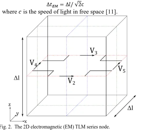
In this paper the TE polarization is assumed for the EM field. The schematic of the TLM node is shown in Fig.2 with transverse electric field components Ex and Ey and a magnetic

field component Hz along the longitudinal z-direction [18].

The node is of the size Δ𝑥 = Δ𝑦 = Δ𝑙 where, in order to minimise the numerical errors, the rule of thumb is that Δ𝑥 is typically less than 𝜆/10 where 𝜆 is the wavelength of the highest frequency of interest[18]. In this manuscript, different mesh sizes were used ranging from 𝜆/10 to 𝜆/20 to avoid the numerical errors that might occur due to modeling frequency dependent materials. The 2D series node has four ports at which it is connected to adjacent nodes and at which the electric fields are related to voltage impulses 𝑉2, 𝑉3, 𝑉4, 𝑉5, as labelled in Fig. 2. The numerical time step is defined as

∆𝑡𝐸𝑀= ∆𝑙/ √2c (5)

where 𝑐 is the speed of light in free space [11].

Fig. 2. The 2D electromagnetic (EM) TLM series node.

The TLM simulation starts with the process of initiation in which incident port voltages are mapped to the nodal voltages. This is followed by a scatter and connect phase as summarized below.

Incident voltages at each node are related to incident port voltages as

[ 𝑉𝑥𝑖

𝑉𝑦𝑖

𝑖𝑧𝑖

] = [10 1

1 0 −1

0 1 −1

0 1 1

] ×

[ 𝑉2𝑖

𝑉3𝑖

𝑉4𝑖

𝑉5𝑖]

, (6)

where 𝑖_𝑧𝑖 is the normalized incident current obtained from 𝑖𝑧= (𝐻𝑧. Δ𝑙. 𝑍𝑜)/√2 and voltage components are related to the electric field as 𝑉𝑥,𝑦 = −𝐸𝑥,𝑦/Δ𝑙.

The total voltage and current at each node are obtained as [

𝑉𝑥

𝑉𝑦

𝑖𝑧

] = [

𝑡𝑒𝑥 0 0

0 𝑡𝑒𝑦 0

0 0 −𝑡𝑚𝑧

] [ 𝑉𝑥𝑖

𝑉𝑦𝑖

𝑖𝑧𝑖

], (7)

where 𝑡𝑒𝑥, 𝑡𝑒𝑦 and 𝑡𝑒𝑧 are the transmission coefficients in x, y and z directions respectively, obtained as [11],

𝑡𝑒𝑥= 𝑡𝑒𝑦=

2

𝑡𝑚𝑧=_{4 + 𝑟} 2 𝑚+ 2𝑠̅𝜒𝑚,

where 𝑠̅ = 𝑗𝜔Δ𝑡 is normalized Laplace variable and 𝜒𝑒, 𝜒𝑚, 𝑔𝑒,𝑟𝑚 are normalised material parameters of electric susceptibility, magnetic susceptibility, electric conductivity and magnetic resistivity, respectively, defined using [11],

𝑔𝑒=𝐺_Δ𝑙𝑒=σ_Δ𝑙e.√2_𝑍 𝑜

𝑟𝑚=𝑅_Δ𝑙𝑚=σ_Δ𝑙m.𝑍𝑜

√2, (9) where 𝜎𝑒, 𝜎𝑚, 𝑍𝑜 are electric conductivity, magnetic resistivity and the impedance of free space, respectively.

In order to incorporate frequency dependent materials into the TLM method, voltages and currents from (7) need to be translated from the frequency domain to the discrete frequency domain. This is done by using the bilinear transform of the form [11],

𝑠̅ = 2 ×1 − 𝑧−1

1 + 𝑧−1 . (10)

In the next stage the voltages and currents of (7) are transformed from the z-domain into the time domain using the inverse Z-transform.

In the scatter phase, the TLM reflected voltages at each port are obtained from the nodal voltages as [11]

[ 𝑉2𝑟 𝑉3𝑟 𝑉4𝑟 𝑉5𝑟]

=

[

𝑉𝑥+ 𝑖𝑧− 𝑉3𝑖 𝑉𝑥− 𝑖𝑧− 𝑉2𝑖 𝑉𝑦− 𝑖𝑧− 𝑉5𝑖 𝑉𝑦+ 𝑖𝑧− 𝑉4𝑖]

.

(11)

In the connection process the reflected voltage pulses of (11) become incident on neighboring ports [11], [18]. The scatter-connect process is repeated for a set number of time-steps or until convergence is reached. A detailed derivation of the TLM method for general dispersive materials is given in [11], [27].

C. The Thermal TLM Model

The thermal TLM model maps the heat conduction equation to a network of transmission lines where each node is represented as a shunt TLM node as shown in Fig.3, [18]. The method maps temperature to voltages, heat flow to currents and a heat source to a current source of the shunt node.

Fig. 3. The 2D thermal TLM shunt node.

The Thevenin equivalent circuit for the 2D shunt thermal model [20] is shown in Fig.4, where incident voltages on each port are 𝑉1𝑖, 𝑉2𝑖, 𝑉3𝑖 and 𝑉4𝑖 and the current source 𝐼𝑠 is placed at the center of the node. The thermal TLM circuit parameters are linked to the material thermal properties through [28],

𝑍 =Δ𝑡

𝐶 =

2Δ𝑡 𝜌𝐶𝑝𝐴Δ𝑙,

(12)

𝑅 = Δ𝑙

2𝐾𝑡ℎ𝐴, 𝑍𝑠=

Δ𝑡 2

1 𝐶𝑠,

where 𝑍 is the characteristic impedance of the transmission line, 𝑅 is the nodal resistance, 𝑍𝑠 is the stub impedance, 𝜌 is mass density, 𝐶𝑝 is the specific heat capacity, 𝐴 = Δ𝑙2 is the nodal area, Δ𝑙 is nodal length, 𝐾𝑡ℎ is the thermal conductivity and 𝐶𝑠 is the stub capacitance evaluated from [28]

𝐶𝑠= 𝐶𝑚− 𝐶𝑏 , (13)

where 𝐶_𝑚 is the material thermal capacitance and 𝐶_𝑏 is the background material thermal capacitance.

Fig. 4. The 2D electromagnetic (EM) TLM series node.

The thermal current source at each node is obtained at every time step from the volumetric dissipated EM power, Pd, as

𝐼𝑠= 𝑃𝑑Δ𝑙 𝐴 (14)

The nodal voltage 𝑉 is then calculated from Thevenin equivalent current as,

𝑉 = 2 ( 𝑉1𝑖

𝑍 + 𝑅 + 𝑉2

𝑖

𝑍 + 𝑅 + 𝑉3

𝑖

𝑍 + 𝑅 + 𝑉4

𝑖

𝑍 + 𝑅 +𝑉𝑠

𝑖

𝑍𝑠) + 𝐼𝑠

4 𝑍 + 𝑅 +𝑍1𝑠

(15)

The reflected voltages on each port are obtained in the scatter stage of the TLM algorithm from [20],

𝑉𝑗𝑟= 𝑉𝑗− 𝑉𝑗𝑖=

𝑍(𝑉−2𝑉_𝑗𝑖)

𝑅+𝑍 + 𝑉𝑗

𝑖_{, j=1,2,3,4 (16)} The total voltage 𝑉𝑗 and current 𝐼𝑗 on each port are found as [20]

𝑉𝑗= 2𝑉𝑗𝑖+ 𝐼𝑗𝑍 = 𝑉 − 𝐼𝑗𝑅, j=1,2,3,4, (17) 𝐼𝑗=

𝑉 − 2𝑉𝑗𝑖

𝑅 + 𝑍 , 𝑗 = 1,2,3,4. (18)

In the connect stage the reflected voltages at each port become incident voltages on the neighboring ports for the next time step. An in the EM TLM algorithm described in section II-D the scatter-connect process is repeated for a required number of time steps or until convergence is reached.

D. Electro-Thermal Coupling

connection between the two domains using the plasma model is described.

There are two principal difficulties in coupling the EM and thermal TLM models. Firstly, the process of switching from a linear material (air) to a nonlinear (plasma) in the time domain requires that the whole process maintains stability and power conservation. Secondly, the time scales, and therefore the simulation time steps of the EM and thermal models, are very different. The simulation time step of the thermal model needs to satisfy [29],

∆tth≪ RthCth, (19)

where RthCth is the lowest product of thermal resistance and the thermal capacitance in the model. Typically due to the slow nature of thermal diffusion compared to the electromagnetic propagation, the thermal time step is much bigger than the EM time step given by (5) (∆tth≫ ∆tEM). In our previous work on modeling plasmonic nano-heat structures[16] it was shown that the thermal and EM time steps do not have to be the same and that computational resources can be saved by setting thermal time steps to be up to 600 times bigger than the EM time step for the same level of accuracy and without affecting the stability of the coupled method.

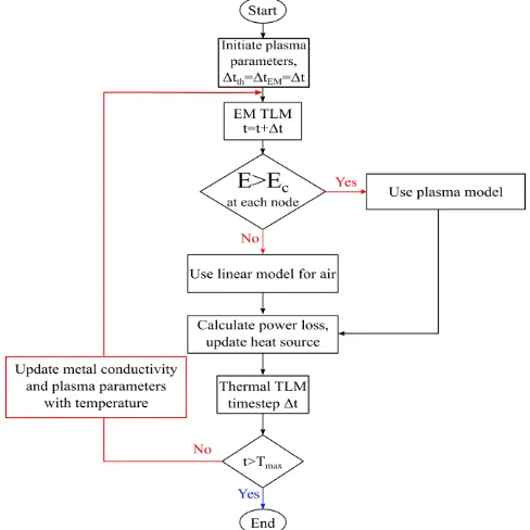
The EM-thermal modelling algorithm is described in Fig.5. For simplicity, the algorithm described assumes the same time step, Δ𝑡 in both domains although this will be further discussed in the results section. The EM TLM model is used to start the propagation of the EM field and set the initial parameters of plasma. As will be described in detail in section III of the present work the source signal takes the form of a double exponential; this is typical of lightning source models. Thus, in the initial stages of the simulation the EM field is relatively low and air is modeled as a linear and uniform material. As the electric field in air builds up, all nodes that have electric field greater than some critical value, 𝐸𝑐, undergo breakdown and become plasma. This requires that the material model in selected spatial nodes is instantly switched from a linear air model to a nonlinear and dispersive plasma model.

The plasma model has a significant conductive component that will cause power loss. At each time step the power loss obtained from the plasma EM model becomes the heat source for the thermal model. In a feedback loop the temperature profile from the thermal model is used to update the electromagnetic properties of the plasma (collision frequency, 𝜈𝑐,plasma frequency, 𝜔𝑝, and particle concentration 𝑛𝑒) and the conductivity of the metal electrodes. Particle concentration dependence on temperature is extracted from [3] for air plasma at atmospheric pressure, using interpolation techniques in order to obtain a continuous curve equation over the entire range of temperature. Using the updated particle concentration and the temperature from the thermal model, collision frequency and plasma frequency are also updated. Similarly, experimental data on the temperature dependent electric conductivity of aluminum was interpolated from [30]. In our earlier experience of modeling arc discharge updating of only the plasma collision frequency was implemented [31]. In this paper the accuracy and suitability of this approach on

the example of arc discharge will be further investigated in the results section.

Fig. 5. The algorithm of the coupling process between electrical and thermal models for the arc discharge.

At every time step the nodal electric and magnetic fields and dissipated power are updated. As the TLM is a time domain method and plasma parameters are defined in the frequency domain, conversion between these two domains needs to be made at every time step. Also, the connection between the electrical and thermal methods needs to be done through plasma model. The imaginary part of the plasma permittivity represents the material conductivity component that is responsible for the power loss in the EM TLM and acts as a heat source in the thermal TLM. The dissipated power loss is related to electric fields in the Laplace domain as [32]

𝑃𝑑(𝑠) = 1

2𝜎𝑒(𝑠)|𝐸̅(𝑠)|2, (20)

where 𝑃𝑑 is the power dissipated per unit volume at a node in W/m3 _and |𝐸̅| is the total electric field in V/m at each node, obtained as |𝐸̅| = √𝐸𝑥2+ 𝐸𝑦2 . Using Parseval’s theorem that states the integral of the function square is equal to the integration of its transform square allows us to transform the dissipated power to Z-domain and then to the digital time domain.

The frequency dependent conductivity 𝜎𝑒 of the plasma in the Laplace domain 𝑠 = 𝑗𝜔 is obtained from (1) and is

𝜎𝑒(𝑠) = 𝜔𝑝2𝜀𝑜 νc+ 𝑠 ,

𝑃𝑑[𝑍] = 1

2𝐾𝑜𝜎𝑜Δ𝑡|𝐸̅[𝑍]|

2_{+ 𝑍}−1 1

𝐾𝑜( 𝜎𝑜Δ𝑡

2 |𝐸̅[𝑍]|2 − (𝐾𝑜−

4

𝜈𝑐) 𝑃𝑑[𝑍]) = 𝛼|𝐸̅[𝑍]|2_{+ 𝑍}−1_{(𝛼|𝐸̅[𝑍]|}2_{+ β𝑃}

𝑑[𝑍])

(22)

where 𝜎_𝑜= (𝜀_𝑜 𝜔_𝑝2)/𝜈_𝑐 denotes the DC conductivity, 𝐾_𝑜 = Δ𝑡 − (2/𝜈𝑐 ) , 𝛼 = (𝜎𝑜 Δ𝑡)/(2𝐾𝑜 ) and 𝛽 = −(1 − 4/(𝐾𝑜𝜈𝑐 )).

The Z-domain description of the dissipated power in plasma in a digital filter representation is given in Fig.6.

Fig. 6. The digital filter used to calculate the frequency dependent dissipated power in plasma.

The inverse Z-transform is used to translate the dissipated power to the time domain as,

𝑃𝑑[𝑛Δ𝑡] = 1

2𝐾𝑜𝜎𝑜Δ𝑡(|𝐸̅[𝑛Δ𝑡]| 2

+ |𝐸̅[(𝑛 − 1)Δ𝑡]|2₎ − 1

𝐾𝑜(𝐾𝑜− 4

𝜈𝑐) 𝑃𝑑[(𝑛 − 1)Δ𝑡]

(23)

𝑃𝑑[𝑛𝛥𝑡] =(|𝐸̅[𝑛𝛥𝑡]|2+ |𝐸̅[(𝑛 − 1)𝛥𝑡]|2)

+ 𝑃𝑑[(𝑛 − 1)𝛥𝑡] (23)

where 𝑛Δ𝑡 represents the current time step, and (𝑛 − 1)Δ𝑡 represents the previous time step. This power is translated to the heat source as in (14) and the updated temperature from the thermal TLM is used to update parameters in the EM TLM method.

III. RESULTS

In this section the coupled EM-thermal model is used to simulate the electric breakdown of air and thermal interaction in the structure shown in Fig.1. In the absence of direct experimental or modeling data we have used this model to investigate the stability and self-consistency of the method and the convergence of results. The method is then applied to the more application oriented case of a diverter strip for lightning strike protection.

The aluminum plates in Fig.1 have the length l=44 mm and width w=18 mm and are separated by a g=18mm air gap. The electrical conductivity of the aluminum plates is taken to be 3.6859 × 107 _{S/m at 25} 𝑜_{𝐶 [30]. A Perfect Electric} Conductor (PEC) boundary condition is placed at the boundaries of the computation space which is of size W=108mm and L=108mm. The voltage source proportional to the 𝐸_𝑥 field component is placed between one of the aluminum plates and the PEC boundary. The source signal has

the form of double exponential waveform [25] typically used to model lightning strike sources and reaches the peak amplitude of 𝑉_𝑐 = 20𝑘𝑉/𝑐𝑚 within 6.5𝜇s and drops down to half the peak value within the next 70𝜇s and is obtained from[25]

𝑉 = 𝑉𝑐× (𝑒−112001 𝑡− 𝑒−670000𝑡) (24) When the electric field in air exceeds the critical value 𝐸𝑐 = 25𝑘𝑉/𝑐𝑚 the air breaks-down [24] and becomes a highly ionized conductive plasma. The critical electric field value at which electric breakdown occurs is dependent on several factors such as the gap width, pressure, air compositions, mass movement and temperature[3]. Considering all of these factors is beyond the work presented in this paper. In this paper only a case of an air gap at atmospheric pressure and ambient temperature is presented and therefore the approximation of critical electric field of 25kV/cm is used [24]. The initial temperature of plasma is taken to be 17000 Kelvin (a typical thermal plasma,≅ 1.5𝑒𝑉) and particle concentration is assumed to be in the range 1 × 1020 < 𝑛𝑒 < 1 × 1024m-3 [3]. The plasma frequency (𝜔𝑝), collision frequency (𝜈𝑒𝑖) and Coulomb logarithm (ln) are calculated based on these initial conditions. Thermal material properties of aluminum, air and plasma, namely specific heat capacity, density and thermal conductivity are summarized in Table 1 [33].

TABLEI.THERMAL MATERIAL PROPERTIES FOR ALUMINUM, AIR AND PLASMA

Material

Properties of the material used in the thermal model

Specific heat capacity J. kg−1_{. K}−1

Thermal conductivity W. m−1_{. K}−1

Density kg. m−3

Aluminum

(Al) 897 237 2707

Air 1005 0.0262 1.2928

Plasma

(at 17000 K) 12696 3.894 5.57× 10

−3

Background 5000 3.894 5.57× 10−3

The results presented in this section compare three ways of coupling between the thermal and EM models. The simplest model assumes no thermal feedback and temperature independent plasma parameters throughout the simulation. The second approach follows the approach presented in [31] for modelling arc discharge in which only plasma collision frequency is updated. The third approach is the full coupled EM-thermal model that updates all temperature dependent parameters of the plasma namely the collision frequency, plasma frequency and particle concentration.

plasma channel for three different spatial discretisations namely, Δ𝑙 = 3.0 mm, Δ𝑙 = 1.8mm and Δ𝑙 = 1.5mm at the simulation time of 9𝜇𝑠. It can be seen that in the case of coarse discretization (Fig.7a) the plasma channel (or lightning spark) is established almost across the entire gap between the metal plates. Finer meshes (Fig.7b, c) show clear separation into two lightning sparks connecting the points with highest field intensity that occur at metal corners due to electric field singularity. Fig.7 confirms that finer discretization provides a better discretization of the arc-like shape of lightning sparks. Based on these results further calculations presented are based on a mesh size of Δ𝑙 = 1.8 𝑚𝑚 which is found sufficient to capture and discuss all important features. In all cases, due to the symmetric nature of the model the arcs are also symmetric across the horizontal axis. It is here emphasized that model does not assume any particular path for the lightning spark and its appearance is defined solely by the strength of the electric field.

Fig. 7. Conducting plasma channel between the aluminum plates for a)

Δ𝑙 = 3.0mm, b) Δ𝑙 = 1.8mm and c) Δ𝑙 = 1.5mm The color scheme (color

online)is blue for air, turquoise for aluminum and yellow for plasma.

Fig.8 analyses how the initial properties of the plasma affect the lightning spark formation. Figs.8(a-c) show arc formation for three different cases of initial electron density typical of a thermal plasma [3] namely 𝑛𝑒= 1 × 1020, 𝑛𝑒= 1 × 1021 and 𝑛𝑒= 1 × 1023 𝑚−3. In all cases the spatial discretization is taken to be Δ𝑙 = 1.8mm and the details of the plasma channel are again taken at the simulation time of 9𝜇𝑠. In this case only the collision frequency is updated with temperature as in [31]. It can be seen that initial conditions for particle concentration can significantly affect the shape of the arcs implying that this parameter has a strong impact on the shape of plasma channel.

Fig. 8. Conducting plasma channel between the aluminum plates when using initial electron density a) 𝑛𝑒= 1 × 1020, b) 𝑛𝑒= 1 × 1021 and c) 𝑛𝑒= 1 × 1023 𝑚−3 for partially coupled model. The color scheme (color

online) is blue for air, turquoise for aluminum and yellow for plasma.

Fig. 9(a-c) show the arc channel formations in the case of fully coupled EM-thermal method where all plasma parameters are updated at every timestep. Three different starting conditions for plasma are considered namely 𝑛𝑒= 1 × 1020 _𝑚−3_{, 𝑛}

𝑒= 1 × 𝑒21 𝑚−3 and 𝑛𝑒= 1 × 1023 𝑚−3. A spatial discretization of Δ𝑙 = 1.8𝑚𝑚 is assumed and the

details of the shape of the plasma channel are taken at simulation time of 9𝜇𝑠. Particle concentration is updated from the experimental data found on page 241 of [3] as explained in II-D, and plasma frequency and collision frequency are updated using (2-4). Fig.9 shows that in all three cases the resulting shape of the arc channel is the same and it can be said that the arc shape has converged with respect to plasma parameters and temperature.

Fig. 9. Conducting plasma channel between the aluminum plates when using initial electron density a) 𝑛𝑒= 1𝑒20m-3, b) 𝑛𝑒= 1𝑒21 m-3 and c) 𝑛𝑒= 1𝑒23 m-3 for fully coupled model. The color scheme (color online) is

blue for air, turquoise for aluminum and yellow for plasma.

Previous results investigate how the shape and position of the lightning channel converge in the model. Figure 10 shows the temperature profile for a plasma node at x=4.68 cm and y=4.68 cm for the mesh size Δ𝑙 = 1.8𝑚𝑚. The initial electron density was taken to be 𝑛𝑒 = 1 × 1021 𝑚−3. Figure.10 compares temperature in the plasma node when: a) there is weak coupling i.e. no update of plasma parameters with temperature throughout the simulation; b) only collision frequency is updated following the work presented in[31] and c) all plasma parameters are updated at every time step. It can be seen that weak coupling of the thermal and EM model predicts much higher temperatures compared to the case when partial or full thermal update of plasma parameters is done. Comparing temperature curves for the partial and full update of plasma parameters we note that in both cases there is a similar prediction for temperature diffusion in plasma, suggesting that both approaches are similar.

Fig. 10. The plasma temperature versus time using different coupling methods.

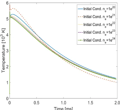
This is further investigated in Figure 11 which compares the case of partial coupling where only collision frequency is being updated for several different starting conditions for plasma particle concentrations (𝑛𝑒= 1 × 1020, 𝑛𝑒= 1 × 1021_{, 𝑛}

the majority of cases the temporal change of temperature follows a similar pattern except for the case of a particle concentration of 𝑛𝑒 = 1 × 1020𝑚−3 (inset of Fig.11) when the method predicts a very different temperature change compared to the other cases where higher electron densities were used as the initial parameter. Note the 1 × 1012 𝐾 temperature scale on the inset. This implies that the stability of the partially coupled EM-thermal method is heavily dependent on the initial parameters and establishes that these parameters should thus be updated during the simulation as in the fully coupled thermal-EM algorithm.

Fig. 11. Temperature profile for a plasma node at x=4.68cm, y=4.68cm using different initial electron concentrations and partially coupled EM-thermal model The instability observed for an initial electron concentration at 𝑛𝑒= 1 × 1020𝑚−3establishes the need for fully coupled thermal-EM model.

The same initial electron density conditions were applied to the fully coupled case where plasma frequency and collision frequency are updated using the temperature profile. The results are shown in Fig.12 showing that the fully coupled model is stable for all initial conditions. Furthermore, the value of the initial condition does not affect the overall behavior of the model.

Fig. 12. Temperature profile for a plasma node at x=4.68cm, y=4.68cm using different initial electron concentrations and fully coupled EM-thermal model

In order to show the convergence of the fully coupled EM-thermal model, the temperature distribution of the plasma channel across the horizontal plane at 𝑦 ≅ 4.68𝑐𝑚 at the simulation time 𝑡 = 0.51𝑚𝑠 is plotted in Fig.13 for different mesh sizes, namely Δl=3.0 mm, 1.8mm and 1.5mm and for an initial electron concentration of 𝑛𝑒 = 1 × 1022𝑚−3. It can be seen that the temperature profile converges as the mesh size decreases and that as mesh size becomes smaller the arc shape becomes more tightly confined. Once again it is seen that a mesh size of Δ𝑙 = 1.8𝑚𝑚 is sufficient.

Fig. 13. Temperature distribution in the plasma region along the horizontal line y=4.68cm

There is an interesting feature in Fig.13 in the line representing mesh size Δ𝑙 = 1.5𝑚𝑚 which is the apparent sudden drop in temperature profile along the y-axis. The reason for this sudden change is the presence in the discretized model of an air node surrounded by plasma. Power dissipation occurs only in plasma nodes meaning the only way for an air node to gain thermal energy is by heat conduction from surrounding plasma nodes. As plasma is a material with much lower density than air the time needed for heat to diffuse from plasma into a neighboring air node is much longer than the simulation time presented here. This demonstrates one of the challenges in modeling the multi-physics features of arc-discharge phenomena and the limitation of the model presented in this paper, as mass transfer and heat convection are important and should be included in the model in order to have a more complete description.

(a)

(b)

Fig. 14. (color online) The temperature profile (a) in the aluminum electrodes (b) in the plasma at 12.22ms

Results reported in Figs.7-14 assume that the time step is set by the requirement of the EM method and that coupling between the EM and thermal model at every time step. For a mesh size Δ𝑙 = 1.8𝑚𝑚 the EM time step is Δ𝑡𝐸𝑀=8.49116ps and the maximum stable time step for the thermal model is Δ𝑡𝑡ℎ= 2.942μs. Running the thermal simulation at the EM time step is computationally expensive. However, the substantial difference between electrical and thermal time steps allows for the thermal model to have the time step as small as the EM time step and up to Δ𝑡𝑡ℎ= 2.942 μs. It is undoubtedly more efficient to run the thermal model using time steps Δ𝑡𝑡ℎ> Δ𝑡𝐸𝑀 whilst guaranteeing that the coupling from the EM to thermal model is done at every Δ𝑡𝑡ℎ.

Fig.15 plots the temperature in the plasma node at x=4.68cm and y=4.68cm using different thermal time steps such that they are integer multiples of the EM time step Δ𝑡𝐸𝑀. The results are shown for time step ratios of Δ𝑡𝑡ℎ/Δ𝑡𝐸𝑀=1, 2, 5, 10 and 100.The results show that actual temperature values in the node are of the same order of magnitude as in the case when Δ𝑡_𝑡ℎ/Δ𝑡_𝐸𝑀=1 but that, unlike the studies reported in [16], Δ𝑡𝐸𝑀 𝑎𝑛𝑑 Δ𝑡𝑡ℎ should remain the same. Figure.16 examines the plasma distribution for the case when Δ𝑡_𝑡ℎ/ Δ𝑡𝐸𝑀=2 and 5. Comparing with Fig.9(c) it can be seen that Fig.16(a) gives different results with much bigger plasma channel as the delay in updating the EM parameters from the thermal model affects the plasma channel formation process. On the other hand Fig.16-b indicates that almost the whole region around the metal plates has turned into plasma. Comparison of the results shown in Fig.9(c) and Fig.16

confirms that for the accurate plasma location prediction the time steps in both models need to be the same.

Fig. 15. Temperature profile for a plasma node at x=4.68cm, y=4.68cm using different time step ratio between EM and thermal model.

Fig. 16. Conducting plasma channel between the aluminum plates when using different timestep ratio for EM and thermal model a) Δ𝑡𝑡ℎ/Δ𝑡𝐸𝑀=2 ;

b) Δ𝑡𝑡ℎ/Δ𝑡𝐸𝑀=5 for the fully coupled model. The color scheme (color

online) is blue for air, turquoise for aluminum and yellow for plasma.

After investigating the validity and convergence of the fully coupled EM-thermal TLM model on a simple example we now apply the model to a simplified case of a diverter strip for lightning protection. Diverter strips are installed on places of high likelihood for lightning strike and are used for lightning protection on aircraft [34]. A diverter strip consists of an insulator layer on top of which conductive segments (square, diamond, circular) are placed and separated by short air gaps. Once lightning hits a diverter strip, a series of cascaded breakdowns occurs in the gaps between the conductive segments with the purpose of drawing the current away from the sensitive electric instruments. The cascade breakdown exhausts the electric field over a distance and limits the destructive capability of the EM field. The simplified (2D) diverter strips geometry studied is shown in Fig.17 and is adopted from [34], where the conductive segments are of square shape with a side length of 3.6mm, the gap between the segments is 0.36mm and the overall problem size is W=20.16mm and L=7.2mm.

Using the similar setup in terms of excitation and boundary conditions as for the air gap model the plasma channel was successively formed between conductive segments and as presented in Fig.18.

(a) 𝑡 = 4.5𝜇𝑠

(b) 𝑡 = 4.755𝜇𝑠

(c) 𝑡 = 4.8824𝜇𝑠

(d) 𝑡 = 4.97𝜇𝑠

Fig. 18. The plasma channel formation in diverter strips using Δ𝑥 =

0.036𝑚𝑚

The fully coupled model is used with an initial electron density of 𝑛_𝑒 = 1 × 1022𝑚−3 and a mesh size of Δ𝑙 = 0.036𝑚𝑚. Fig.18 shows a cascade of lightning arcs that are formed at the corners of the metal plates.

IV. CONCLUSION

A stable electromagnetic EM-thermal multi-physics coupled model for modeling lightning arcs induced by the presence of a strong electric field is demonstrated. Lightning arcs are modeled as a conductive plasma channel where a frequency dependent Drude model is used for the plasma material model.

The model makes no assumptions on the physical location of the lightning channel but predicts its appearance purely from the electromagnetic field conditions. Power loss in the EM model is used as the heat source for the thermal model at regular time intervals. It has been shown that stability issues require that the timesteps of both EM and thermal are kept the same. The results show that full thermal feedback from the thermal method to the EM method that updates all plasma parameters with temperature, namely plasma frequency, collision frequency and particle concentrations, is necessary for the convergence of both the shape and temperature of the plasma channel. The method is extended to the example of a diverter strip and it is shown that the lightning path is propagating away from the source and connects the points of highest electric field in the model.

REFERENCES

[1] P. K. Mallick, Fiber-reinforced composites: materials,

manufacturing, and design. CRC press, 2007.

[2] H. B. Cary, Modern welding technology. Prentice-Hall, 1979. [3] Maher I.Boulos, P. Fauchais, and E. Pfender, Thermal Plasmas

Fundamentals and Applications Volume 1. New York: Plenum

Press, 1994.

[4] L. Niemeyer, L. Pietronero, and H. J. Wiesmann, “Fractal Dimension of Dielectric Breakdown,” Phys. Rev. Lett., vol. 52, no. 12, pp. 1033–1036, Mar. 1984.

[5] A. Luque and U. Ebert, “Growing discharge trees with self-consistent charge transport: the collective dynamics of streamers,”

New J. Phys., vol. 16, no. 1, p. 013039, Jan. 2014.

[6] J. Wendelstorf, “Ab initio modelling of thermal plasma gas discharges( electric arcs ),” Braunschweig University of Technology, 2000.

[7] M. S. Benilov, “Understanding and modelling plasma–electrode interaction in high-pressure arc discharges: A review,” J. Phys. D.

Appl. Phys., vol. 41, no. 14, p. 144001, Jul. 2008.

[8] M. Tanaka and J. J. Lowke, “Predictions of weld pool profiles using plasma physics,” J. Phys. D. Appl. Phys., vol. 40, no. 1, pp. R1– R23, Jan. 2007.

[9] M. A. Da Frota Mattos and C. Christopoulos, “A nonlinear transmission line model of the lightning return stroke,” IEEE Trans.

Electromagn. Compat., vol. 30, no. 3, pp. 401–406, 1988.

[10] R. J. Luebbers, F. Hunsberger, and K. S. Kunz, “A frequency-dependent finite-difference time-domain formulation for transient propagation in plasma,” IEEE Trans. Antennas Propag., vol. 39, no. 1, pp. 29–34, 1991.

[11] J. Paul, “Modelling of general electromagentic material properties in TLM, PhD thesis,” Univeristy of Nottingham, 1998.

[12] H. Tsubata, T. Nishi, H. Fujisawa, Y. Baba, and M. Nakagawa, “FDTD simulation of lightning current in a multi-layered CFRP material,” in International Conference on Lightning & Static

Electricity (ICOLSE 2015), 2015, p. 16 (4 .)–16 (4 .).

[13] R. B. Neufeld, “Lightning direct effects on anisotropic materials from electro-thermal simulation,” in International Conference on

Lightning & Static Electricity (ICOLSE 2015), 2015, no. 2, p. 7 (5

.)–7 (5 .).

[14] T. Ogasawara, Y. Hirano, and A. Yoshimura, “Coupled thermal– electrical analysis for carbon fiber/epoxy composites exposed to simulated lightning current,” Compos. Part A Appl. Sci. Manuf., vol. 41, no. 8, pp. 973–981, Aug. 2010.

[15] G. Abdelal and A. Murphy, “Nonlinear numerical modelling of lightning strike effect on composite panels with temperature dependent material properties,” Compos. Struct., vol. 109, no. 1, pp. 268–278, Mar. 2014.

[16] A. Elkalsh, A. Vukovic, P. D. Sewell, and T. M. Benson, “Electro-thermal modelling for plasmonic structures in the TLM method,”

Opt. Quantum Electron., vol. 48, no. 4, p. 263, 2016.

infrared: Al, Co, Cu, Au, Fe, Pb, Mo, Ni, Pd, Pt, Ag, Ti, V, and W,”

Appl. Opt., vol. 24, no. 24, p. 4493, Dec. 1985.

[18] C. Christopoulos, The Transmission-Line Modeling Method TLM. New York, USA: IEEE press, 1995.

[19] H. C. Patel, “Non-linear 3D modelling heat of flow in magneto-optic multilayered media,” University of Keele, 1994. [20] D. DeCogan, Transmission Line Matrix (TLM) techniques for

diffusion applications. Amesterdam, The Netherlands: Gordon and

Breach Science Publishers, 1998.

[21] R. Hocine, A. Boudghene Stambouli, and A. Saidane, “A three-dimensional TLM simulation method for thermal effect in high power insulated gate bipolar transistors,” Microelectron. Eng., vol. 65, no. 3, pp. 293–306, Mar. 2003.

[22] C. Flockhart, “The simulation of coupled electromagnetic and thermal problems in microwave heating,” in Second International

Conference on Computation in Electromagnetics, 1994, vol. 1994,

no. 4, pp. 267–270.

[23] E. W. Williams, H. C. Patel, D. De Cogan, and S. H. Pulko, “TLM modelling of thermal processes in magneto-optic multi-layered media,” J. Phys. D. Appl. Phys., vol. 29, no. 5, pp. 1124–1132, May 1996.

[24] V. Cooray, The Lightning Flash, 1st ed. The Institution of Engineering and Technology, Michael Faraday House, Six Hills Way, Stevenage SG1 2AY, UK: IET, 2003.

[25] W. Jia and Z. Xiaoqing, “Double-exponential expression of lightning current waveforms,” in The 2006 4th Asia-Pacific

Conference on Environmental Electromagnetics, 2006, pp. 320–

323.

[26] D. M. Goebel and I. Katz, Fundamentals of Electric Propulsion: Ion

and Hall Thrusters. Hoboken, NJ, USA: John Wiley & Sons, Inc.,

2008.

[27] J. Paul, C. Christopoulos, and D. W. P. Thomas, “Generalized material models in TLM .I. Materials with frequency-dependent properties,” IEEE Trans. Antennas Propag., vol. 47, no. 10, pp. 1528–1534, 1999.

[28] H. R. Newton, “TLM models of deformation and their application to vitreous china ware during firing,” The University of Hull, 1994. [29] D. De Cogan and A. De Cogan, Applied Numerical Modelling for

Engineers. Oxford: Oxford Univeristy Press, 1997.

[30] P. D. Desai, H. M. James, and C. Y. Ho, “Electrical resistivity of aluminum and manganese,” J. Phys. Chem. Ref. Data, vol. 13, no. 4, p. 1131, 1984.

[31] A. Elkalsh, A. Vukovic, P. Sewell, and T. M. Benson, “Coupled arc discharge models in the TLM method,” in 2015 IEEE International

Symposium on Electromagnetic Compatibility (EMC), 2015, pp.

987–990.

[32] S. J. Orfanidis, Electromagnetic Waves and Antennas. 2014. [33] W. Benenson, J. W. Harris, H. Stocker, and H. Lutz., Eds.,

Handbook of Physics, 1st ed. New York: Springer-Verlag, 2002.

[34] N. I. Petrov, A. Haddad, G. N. Petrova, H. Griffiths, and R. T. Waters, “Study of Effects of Lightning Strikes to an Aircraft,” in

Recent Advances in Aircraft Technology, InTech, 2012.

Ahmed Elkalsh was born in Kuwait in 1989. He

received the bachelor’s degree in electronic and communication engineering (BEng Hons) from University of Nottingham, Nottingham, U.K. in 2012.

He is currently working toward the PhD. Degree in electrical and electronic engineering at the University of Nottingham where he is currently working as a research fellow. His research interest include Multiphysics numerical modeling, lightning, complex materials and optoelectronics.

Phillip Sewell (M’89-SM’04) was born in London,

U.K., in 1965. He received the B.Sc. degree in electrical and electronic engineering (with first-class honors) and Ph.D. degree from the University of Bath, Bath, U.K., in 1988 and 1991, respectively. From 1991 to 1993, he was a Post-Doctoral Fellow with the University of Ancona, Ancona, Italy. In1993, he became a Lecturer with the School of Electrical and Electronic Engineering, University of Nottingham, Nottingham, U.K. In 2001 and 2005, he

became a Reader and Professor of electromagnetics at the University of Nottingham. His research interests involve analytical and numerical modeling of electromagnetic problems with application to opto-electronics, microwaves, and electrical machines.

Trevor M. Benson received a First Class honors

degree in Physics and the Clark Prize in Experimental Physics from the University of Sheffield in 1979, a PhD in Electronic and Electrical Engineering from the same University in 1982 and the DSc degree from the University of Nottingham in 2005.

After spending over six years as a Lecturer at University College Cardiff, Professor Benson moved to The University of Nottingham in 1989. He was promoted to a Chair in Optoelectronics in 1996, having previously been Senior Lecturer (1989) and Reader (1994). Since October 2011 he has been Director of the George Green Institute for Electromagnetics Research at The University of Nottingham. Professor Benson’s research interests include experimental and numerical studies of electromagnetic fields and waves with particular emphasis on the theory, modeling and simulation of optical waveguides, lasers and amplifiers, nano-scale photonic circuits and electromagnetic compatibility.

He is a Fellow of the Institute of Engineering Technology (FIET) and the Institute of Physics (FInst.P). He was elected a Fellow of the Royal Academy of Engineering in 2005 for his achievements in the development of versatile design software used to analyze propagation in optoelectronic waveguides and photonic integrated circuits

Ana Vukovic (M’97) was born in Nis, Yugoslavia,

in 1968. She received the Diploma of Engineering degree in electronics and telecommunications from the University of Nis, Nis, Yugoslavia, in 1992, and the Ph.D. degree from the University of Nottingham, Nottingham, U.K., in 2000.