A changepoint analysis
of spatio-temporal point processes
Linda Altieri1,∗, E. Marian Scott2,, Daniela Cocchi1,, Janine B. Illian3,
Abstract
This work introduces a Bayesian approach to detecting multiple unknown
change-points over time in the inhomogeneous intensity of a spatio-temporal point
pro-cess with spatial and temporal dependence within segments. We propose a new
method for detecting changes by fitting a spatio-temporal log-Gaussian Cox
pro-cess model using the computational efficiency and flexibility of integrated nested
Laplace approximation, and by studying the posterior distribution of the
po-tential changepoint positions. In this paper, the context of the problem and
the research questions are introduced, then the methodology is presented and
discussed in detail. A simulation study assesses the validity and properties of
the proposed methods. Lastly, questions are addressed concerning potential
un-known changepoints in the intensity of radioactive particles found on Sandside
beach, Dounreay, Scotland.
Keywords: spatio-temporal point processes, changepoint analysis, INLA,
radioactive particle data
2014 MSC: 00-01, 99-00
∗Corresponding author
Email address: [email protected](Linda Altieri) 1University of Bologna, Department of Statistical Sciences 2University of Glasgow, School of Mathematics and Statistics
1. Introduction
In this work, we propose a method for carrying out a changepoint analysis
in the complex context of temporal point processes. Increasingly,
spatio-temporal point process data are becoming routinely available allowing questions
concerning changes in the intensity of the process to be addressed, such as
5
in earthquake studies, where locations of earthquake epi-centres and strength
are mapped over time and where there is an interest assessing changes in the
intensity and spatial distribution of seismic events over recent years [1, 2], or
in occurrence of conflict data [3]. Other case studies derive from the field of
environmental monitoring, such as the dataset presented here.
10
Our study is motivated by questions on the monitoring and recovery of
ra-dioactive particles from Sandside beach, North of Scotland, close to the former
Dounreay nuclear facilities [4].Minute fragments of irradiated nuclear fuel
par-ticles, generally similar to grains of sand, have been generated by historic
prac-tices at UKAEA Dounreay (http://www.dounreay.com/particle-cleanup).
15
UKAEA Dounreay historically released particles primarily into the marine
envi-ronment Since 1984, particles have been found on the publicly accessible beach
at Sandside Bay. A variety of different monitoring systems have been used
and the frequency of monitoring has also varied over the period since routine
monitoring first began. The beach monitoring campaign has several purposes,
20
primarily driven by the recovery of particles, and thus reduction of risk to the
public from encountering such particles and hence public reassurance. At the
same, it provides improved understanding and knowledge of the particle
popula-tion abundance and its change as a result of continued monitoring and retrieval
of particles offshore and historic site practices. Monitoring of the beaches (and
25
in particular Sandside beach) has been ongoing for a number of years with the
first particles being detected in the 1980s. Over the past 15 years, two
ma-jor changes in the equipment used to detect the onshore particles have taken
place, representing known potential changepoints. In addition, offshore particle
retrieval campaigns are believed to have reduced the particle intensity for
ticles moved onshore with tides and currents with an unknown temporal lag,
potentially generating multiple unknown changepoints in the intensity function
of the particle distribution. Questions on how to construct a method able to
de-tect unknown changepoints in such a complex dataset are raised; the proposed
method has to deal with the issues of spatial inhomogeneity, spatial dependence
35
among points and temporal dependence of the process.
1.1. Background and tools
For our work, we use a class of point process models called log-Gaussian
Cox Processes (LGCPs). Cox processes assume that the point distribution over
space is due to stochastic environmental heterogeneity, modelled as a random
40
intensity function; given a realisation of the intensity surface, the distribution of
points follows an inhomogeneous Poisson process. In LGCPs, the logarithm of
the intensity surface over an observation windowW is assumed to be a (latent)
Gaussian random field. For a review on point process models and LCGPs we
refer to [5] and [6]. LGCPs constitute a very flexible class of models that can
45
potentially be extended to spatio-temporal data [7]; tractability issues that have
impeded the use of these models up to very recent years can now be overcome
using Integrated Nested Laplace Approximation (INLA, [8]).
INLA is an alternative option to MCMC methods for approximating the
pos-terior distribution of the parameters of interest; it is simulation free, which
50
is the key to its speed, and it exploits two approximations. Firstly, a Laplace
approximation is employed to represent the posterior distributions with a
Gaus-sian shape; secondly, the GausGaus-sian Field is substituted by a GausGaus-sian Markov
Random Field with a sparse precision matrix, which makes calculations very
efficient. INLA returns the posterior probability of every time point of being a
55
changepoint, allowing the changepoint positions to be inferreda posteriori.
Changepoint analysis is a well-established area of statistical research, frequently
applied in a temporal context, and less frequently over space [9]. The basic
as-sumption is that data are ordered and split into time segments following the
same model but under different parameter specifications [10]; the other
mon assumption is that observations arei.i.d.. The interest lies in detecting the
time and magnitude of the change(s). For a review of changepoint techniques
for temporal data we refer to [11]. We aim at understanding what happens
when the usual assumptions of a changepoint analysis (simply temporal i.i.d.
data) do not hold, which raises a few challenging issues especially when applied
65
to the context of point processes.
1.2. Theoretical issues
While some of the existing changepoint methods can potentially be extended
to the general spatio-temporal context, for spatio-temporal point processes this
branch of analysis appears to be as yet relatively unexplored. Some
substan-70
tial differences with regard to the standard changepoint analysis in time or in
space have to be taken into account: firstly, at every time point the datum is
not a single point but an irregular pattern of points, distributed over a
pos-sibly irregular observation window. Secondly, in many real situations, spatial
dependence among points and temporal dependence within time segments have
75
to be taken into account, and analytically obtaining mathematical quantities
of interest, such as likelihood values and posterior distributions, is not trivial;
modelling dependence within data segments in the context of unknown multiple
changepoints is currently a challenge even for simple temporal series. Thirdly,
frequently point process data are collected over space, and it is not common
80
to have repeated measurements in the same observation window over time, in
a sequence large enough to allow changepoint analysis. Most of the studies on
point processes aim at describing the behaviour of the intensity function,
there-fore its changes over time are certainly of interest, and the provision of tools for
changepoint analysis on spatio-temporal processes would enlarge the number
85
of questions that can be answered, especially when spatial dependence among
points and temporal dependence within time segments are included.
1.3. Research questions
The aim of our work is to propose a method to find multiple unknown
changepoints over time in the inhomogeneous intensity of a spatio-temporal
point process, allowing for spatial and temporal dependence within segments.
When dependence is allowed, the segment marginal likelihood usually becomes
intractable, hence there is a need for fast computational methods, such as INLA,
providing an accurate and tractable approximation of the likelihood. The
com-putational speed and flexibility of INLA has not yet been exploited for a
spatio-95
temporal changepoint analysis.
When applied to spatio-temporal point processes, a changepoint analysis of
the behaviour of the intensity function over time can address different aspects:
firstly, a change in scale, when the overall number of points increases or
de-creases significantly after a certain time point. Another option is a change in
100
spatial structure, when the expected number of points remains constant, but
their distribution over space changes after a certain time point. Lastly, the
change can occur in both scale and spatial distribution. In the special case of a
change in scale only, and when spatial homogeneity can be assumed throughout
the whole time series, our method reduces to a traditional changepoint analysis
105
on the time series of point counts. Our method allows changepoint detection
to be extended to any point process where the information concerning the
spa-tial distribution is of interest (as in the examples at the beginning of Section 1
state).
We aim at developing a method that is able to detect any of these changes
110
over time, and that can therefore provide answers to a wider variety of cases
and carry much more information than a traditional changepoint analysis that
ignores spatial structure.
1.4. Motivation for the approach
In this study, we take a Bayesian approach to changepoint analysis for two
115
main reasons. First of all, Bayesian inference allows knowledge brought by data
(the likelihood) to be enriched by including extra information in the prior
dis-tributions of the parameters; in many real situations some changepoints might
be considered more likely than others. Secondly, a Bayesian approach allows
dependence to be dealt with, while there are currently no satisfactory
tist solutions to the problem.
We use INLA to fit latent Gaussian models such as LGCPs as it brings
substan-tial advantages when it comes to detecting multiple changepoints in a
spatio-temporal point process context: first of all, very complex models can be fitted
using INLA; the extension to spatio-temporal models is computationally
chal-125
lenging but feasible, and accurate and tractable approximations of the segment
marginal likelihoods can be produced. Secondly, we can explore all the time
series and compare the likelihood values resulting from different changepoint
positions to choose the best positiona posteriori. This is more efficient than
traditional changepoint algorithms [11]; such a complex exploration in such a
130
complex dataset would not be possible in reasonable time without INLA.
2. Methodology
2.1. Models
We consider a changepoint under four increasingly complex point process
models, and consider the case of both a single changepoint and multiple
change-points at unknown locations; we discretise the observation window into a fine
grid, and defineyts∼P oi(|C|λts) as the number of points at timet= 1, . . . , T
in cells= 1, . . . , S, where|C| is the cell area. As is traditional in changepoint
analysis [ref], we present the changepoint search as a test of two alternative
hy-potheses. H0 means no changepoint;H1only concerns the number (1 or more)
of changes and is therefore a complex hypothesis that may be decomposed in
different sub-hypotheses for different changepoint positions.
We initially consider a model (Model 1) with an intercept, which assumes a
spa-tially homogeneous intensityλt; under each hypothesis (for the alternative, the
case of a single changepoint is displayed for simplicity) we model the logarithm
of the intensity functionλtas:
H0: log(λt) =µ+t fort= 1, . . . , T
H1: log(λt) =µ1+t fort≤θ∗
log(λt) =µ2+t fort > θ∗
where µ is the intercept and t ∼ iidN(0, τ) is an unstructured error term.
Under H0 all values over both space and time depend on a single value for µ,
while underH1 µtis constant over space but allowed to vary over time: a
sin-gle changepoint in locationθ∗ splits the dataset into two time segments with a
different value for the intensity function. In the more general case of M ≥ 2
changepoints, the equation underH1 is split intoM + 1 segments defined by
the ordered changepoint locationsθ1, θ2, . . . , θM.
Extensions to Model 1 (Equation (1)) include adding a temporal effect (Model
2) and an extension to inhomogeneous processes (allowing for a spatially
inho-mogeneous intensity functionλts) by including a spatial effect (Model 3). All
effects are included in Model 4 (given in Equation 2).
H0: log(λts) =µ+φ+ψs+ts fort= 1, . . . , T and s= 1, . . . , S
H1: log(λts) =µ+φ1+ψ1s+ts fort≤θ∗ ands= 1, . . . , S
log(λts) =µ+φ2+ψ2s+ts fort > θ∗ ands= 1, . . . , S
(2)
µis a common intercept and, within each time segment, φ is a random effect
modelled as an AR(1): φt=φt−1+utwhereut∼N(0, τφ−1). Priors are needed
135
for the precision τφ ∼ Gamma(αφ, βφ). The spatial effect is ψs where the
basic space unitsis the grid cell. This approximation is needed for tractability
reasons, but INLA allows extremely fine grids while still being computationally
feasible. ψs is modelled as an intrinsic CAR, i.e. as a Random Walk in two
dimensions on a lattice, with a smooth neighbourhood structure that gives
non-140
zero weights to the first 12 neighbours in the lattice [12]. Again, the precision
hyperparameter can be defined asτψ∼Gamma(αψ, βψ).
The current implementation of INLA in the R-INLA software (www.r-inla.org)
is not restricted to the spatial and temporal random fields chosen here.
2.2. Single changepoint detection
145
The single changepoint detection procedure starts by comparing the
sub-hypotheses underH1, obtaining the marginal likelihoods conditional on different
the likelihood underH0, or compared to a chosen threshold. To do this, we now
present two different Bayesian techniques.
150
2.2.1. Bayes Factor method
We propose a modified version of the logarithm of the Bayes Factor, with
only one term forθ∗ instead of all possibleθs:
γθ0∗= log(π(θ∗)) +q1(θ∗) +q2(θ∗)−l0= log(π(θ∗)) +l1(θ∗)−l0. (3)
whereθ∗ is the changepoint position returning the highest likelihood value
un-der H1, π(θ∗) is the value of the prior distribution at the changepoint, and
l1(θ∗) =q1(θ∗) +q2(θ∗) is the corresponding maximum log-likelihood under the
alternative hypothesis, obtained as a sum of two segment log-likelihoods. For
155
the model with no changepoints, the maximum log-likelihood value underH0is
greater than the maximum log-likelihood value underH1, as Bayes factors
nat-urally incorporate penalization for model complexity. Ifγ0θ∗>0, we reject the
null model of no changepoint, and the changepoint is estimated to occur atθ∗.
In conclusion, this method first compares the options underH1 and then tests
160
the best one againstH0and is routinely used in Bayesian temporal changepoint
analysis [11].
2.2.2. Posterior Threshold method
An alternative option is to fix a posterior probability threshold to identify
changepoints. We consider the posterior distribution of the changepoint
posi-165
tions coming from the likelihood values conditional on different options under
H1. Instead of testing them againstH0, we use a decision threshold: if there are
peaks in the posterior distribution above the threshold, the highest peak
corre-sponds to the accepted changepoint. Suggestions for the choice of the threshold
are given in Section 5. This method has the advantage of being visually
im-170
mediate and easy to explain to non-statisticians; moreover, it is very flexible as
the threshold choice can be adapted to the model fitting the data and to the
2.3. Multiple changepoint detection
We now extend the method to an unknown number of changepoints; two
175
approaches can be taken: a binary segmentation algorithm aimed at finding
one changepoint in each step, or a simultaneous search aiming at finding all
changepoints in one step.
2.3.1. Binary segmentation algorithms
For a general introduction to these methods we refer to [11], and in
partic-180
ular for point processes to [13]. The idea of a binary segmentation procedure,
and the key to its simplicity, is to split the multiple search into a series of
sub-sequent searches; in each step, a single changepoint search is carried out, and
either method (BF or PT) can be used. When running such an algorithm,
num-ber and positions of changepoints are estimated sequentially at the same time:
185
in each step, if a changepoint is found, its position is immediately chosen before
moving on to the next step, as we need to know where to split the data into
further segments.
The analysis can become computationally very demanding asT andM become
large, and methods are available for reducing time and memory storage
require-190
ments [11]. The computational efficiency of INLA makes this algorithm feasible
even for complex spatio-temporal data.
2.3.2. Simultaneous changepoint search
The procedure we build follows a two level prior setting as in [14] and [15],
where a prior distribution is given to the number of changepoints and then a
195
prior conditional on the number is given to the changepoint locations. As a
consequence, we first estimate the number of changepoints, then conditional on
that we identify the most likely positions. We then follow [14] with an extension
to spatio-temporal models. M + 1 conditional likelihoods are computed using
recursive equations, which give evidence for the model with m changepoints,
200
m= 0, . . . , M. Ifπ(M) is non informative, the highest likelihood valueL(Y|m)
2.4. Posterior distribution
Irrespective of the detection method, the final goal of a Bayesian changepoint
analysis is to obtain a posterior distribution of the number and positions of
205
changepoints.
In a single changepoint search, the algorithm produces a posterior distribution
assigning a probability to every potential changepoint position. For each model
scenario, we run the modelT times under the alternative hypothesis. In each
run, we condition on the changepoint occurring at a different specific location
210
θ∈ {1, . . . , T} and fit one of the models; we obtain a conditional log-likelihood
valuel1(θ) = q1(θ) +q2(θ) (see Section 2.2.1). TheT-dimensional vectorl1 =
{l1(θ), θ ∈ {1, . . . , T}} is then transformed following the usual Bayes Rule to
obtain the posterior distribution: in the absence of prior knowledge, rescaling
the likelihood vector to integrate to 1 gives the posterior distribution of interest.
215
The time point corresponding to the maximum posterior value is taken as the
most likely changepoint positiona posteriori θ∗. The decision on the significance
of the detected potential changepoint with respect to the null hypothesis can
be based on either the Bayes Factor or the Posterior Threshold method. The
computational expense of refitting each model many times for different potential
220
changepoints is not prohibitive when using INLA.
In a multiple changepoint search, as for the binary segmentation algorithm,
a criterion for decision making must be chosen first in order to proceed with
the iterations. Any of the methods proposed in 2.2 can be used; once chosen,
the posterior distribution for each potential changepoint position is obtained for
225
each step and time segment just as for the single search. Since time is discrete, a
final posterior distribution for the whole time series can be obtained by averaging
values pointwise and then rescaling in order to integrate to 1 and to deal with
a proper distribution. If a simultaneous search is carried out, we obtainM + 1
conditional data likelihoodsL(Y|m= 0),L(Y|m= 1), . . . ,L(Y|m=M), where
230
Y is the whole dataset. Following the Bayes Rule P(m|Y) ∝L(Y|m)π(m), if
the prior is uniform ˆM = arg maxm{L(Y|m),m= 1, . . . , M}. Conditional on
ˆ
previous change (with the conventionθ0 = 0), the data and ˆM. Assuming the
changepoint process is a Markov process we find them iteratively:
235
P(θ1, . . . , θMˆ|Y,Mˆ) =P(θ1|Y,Mˆ)×P(θ2|θ1, Y,Mˆ)× · · · ×P(θMˆ|θMˆ−1, Y,Mˆ).
3. Simulation study
In order to assess and compare the performance of the methods proposed in
Section 2.1, we carry out a simulation study covering different situations.
3.1. Simulation design
240
We fix a time series of T = 50 time points, and a grid of S = 20×20 =
400 cells. The observation window W is a square of area 100. We also ran
simulations in irregular polygonal windows, which did not lead to substantially
different conclusions; we therefore only consider the square window here.
We simulate point pattern data that follow an i.i.d. and an AR(1) process in
245
time, respectively, for both single and multiple changepoint detection underH0
(no changepoint, λ= 1 over the whole series) and under different options for
H1:
• one large changepoint in scale (fromλ1= 1 toλ2= 2)
• one small changepoint in scale (fromλ1= 1 toλ2= 1.2)
250
• three changepoints in scale (λ1= 1, λ2= 1.4,λ3= 2.3,λ4= 2)
• one changepoint in spatial structure
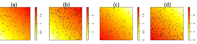
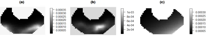
• one changepoint in both scale and spatial structure.
Figure 1 shows examples of the above listed changes. Panel (a) displays the
initial value for the intensity function; panel (b) shows a large change in scale
255
(small change and multiple changes not displayed here); panel (c) a change in
spatial structure; panel (d) a change in both space and scale.
Data with a change in scale are generated under both a homogeneous (a single
Figure 1: Examples of simulated data, with the corresponding underlying intensity function:
initial intensity (a), large scale change (b), spatial change (c), spatial and scale change (d)
forλsover the window, with a mean value over space equal to the homogeneous
260
λ). 100 replicates are generated for each case.
In order to find a sensible and not too arbitrary threshold for the PT method,
it is possible to use simulated data under the null hypothesis for assessing the
significance level αbased on different threshold values. Once we find a value
such that the significance level does not exceed a certain limit (usually α ≤
265
{0.01,0.05,0.1}), we use that threshold on data generated under the alternative
hypothesis in order to evaluate its power level, the ability to detect the correct
changepoint locations and the accuracy of the produced estimates.
3.2. Simulation results
After we fit Model 1 to 4 (Section 2.1) to all simulated patterns, we assess
270
the performance of the proposed detection techniques: for a single search, the
BF and PT methods (2.2); for a multiple search, the simultaneous approach and
the binary segmentation algorithm combined with both BF and PT methods
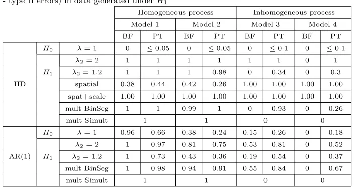
(2.3). Methods are evaluated based on type I and type II errors (see Table
1), number and position of detected changepoints and accuracy of the intensity
275
estimates (tables not reported here). Table 1 does not report results where the
data generation process and the nature of the model do not match: Model 1
and 2 are appropriate for spatially homogeneous data, while Model 3 and 4 are
only relevant to inhomogeneous data.
As for the ability to detect changepoints (i.e.to rejectH0), Table 1 shows that
Table 1: ’Significance levels’ (type I errors) in data generated underH0and ’power levels’ (1
- type II errors) in data generated underH1
Homogeneous process Inhomogeneous process
Model 1 Model 2 Model 3 Model 4
BF PT BF PT BF PT BF PT
IID
H0 λ= 1 0 ≤0.05 0 ≤0.05 0 ≤0.1 0 ≤0.1
H1
λ2= 2 1 1 1 1 1 1 0 1
λ2= 1.2 1 1 1 0.98 0 0.34 0 0.3
spatial 0.38 0.44 0.42 0.26 1.00 1.00 1.00 1.00
spat+scale 1.00 1.00 1.00 1.00 1.00 1.00 1.00 1.00
mult BinSeg 1 1 0.99 1 0 0.93 0 0.26
mult Simult 1 1 0 0
AR(1)
H0 λ= 1 0.96 0.66 0.38 0.24 0.15 0.26 0 0.18
H1
λ2= 2 1 0.97 0.81 0.75 0.53 0.81 0 0.52
λ2= 1.2 1 0.73 0.43 0.36 0.19 0.54 0 0.37
mult BinSeg 1 0.98 0.94 0.91 0.55 0.84 0 0.67
mult Simult 1 1 0 0
when a change in scale is considered all methods perform quite well over the
first two models, but all detection techniques that use the BF method and the
simultaneous search become too conservative as soon as spatial dependence is
included (too many 0s in the table); the PT method performs better over all
models, also due to the possibility to tune the threshold value according to the
285
model. We also covered different types of change in the intensity function which
involve the spatial distribution (labelled as ’spatial’ and ’spat+scale’ in Table
1). When a single change in spatial structure is considered, the performance
of all methods is excellent: changes in the spatial structure are detected with
both methods when using Models 3 and 4, which include a spatial effect, and
290
changes in both scale and space are detected for all models.
Once the ability to reject H0 is assessed, we focus on the number of detected
changepoints. Results are correct in allH0data: even in situations where some
changepoints were found, as in AR(1) data, they were correctly identified as
spurious changepoints (in a different location for every replicate). As regards
295
the detection in H1 data, when a changepoint is detected with any method,
changepoint that the slight mislocation would be irrelevant in practice. Again,
spurious changes in time dependent data do not affect the conclusions,i.e.our
methods are still able to detect the correct changepoint locations despite the
300
variability in the time series.
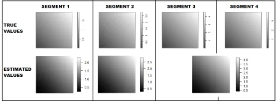
Lastly, given the detected changepoints, estimates are very accurate over all
the simulated scenarios; see Figure 2 for an example. When a changepoint
is not detected (e.g. third/fourth column in Figure 2), estimated values are
located in between the two segments’ true values, and when a changepoint was
305
only detected in a proportion of the replicates (as happens with very small
changes), the true magnitude of the change is reduced. When a change in scale
is considered, the correct (increasing or decreasing) trend is always captured; as
can be seen from Figure 2, results are very accurate in reproducing both scale
[image:14.612.165.443.364.468.2]and spatial trend.
Figure 2: Simulated intensity functions for four time segments, with three changepoints (top
panels) - Estimated segment intensities under the detection of two changepoints (bottom
panels)
310
4. Case study
Since the 1950s, Dounreay has been the site of several nuclear research
estab-lishments, most of which are now being decommissioned. Radioactive particles
have been found on local beaches in the North of Scotland since the 1990s as
a result of historic practices during nuclear fuel reprocessing at the Dounreay
plant (http://www.dounreay.com). The dataset used gives the particles’
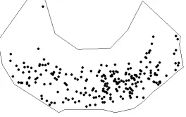
loca-tions on one of the local beaches, Sandside beach, during each of the years of
monitoring [16] (see Figure 3). The temporal data series consists of yearly point
pattern realizations, and additional information on the retrieval and
radioac-tivity level for each of the particles. The underlying intensity and its spatial
320
structure are of interest, along with potential changes. For the questions
pre-sented in Section 1, this motivating dataset represents an adequate example of
an inhomogeneous spatio-temporal point process with changepoints over time.
[image:15.612.239.371.296.379.2]MCMC goodness of fit tests [5] show that Cox processes fit data very well;
Figure 3: Radioactive particles detected on the Sandside beach between 1999 and 2013
in particular, the flexible class of log-Gaussian Cox processes is suitable for the
325
problem as the distribution of particles could be due to an underlying driver
(tides and winds). Moreover, it is very straightforward to modify these models
by adding an intercept, random or smooth effects to the structured predictor;
the estimation with INLA is very fast (and precise) even for complex models and
this allows us to fit several different models without becoming computationally
330
prohibitive.
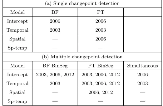
4.1. Results on particle data
Table 2 displays a summary of the number and positions of detected
change-points in the data series for both a single and a multiple search. Results must
be interpreted carefully since the time series is very short. The first two
de-335
tected changepoints in 2003 and 2006 correspond to the periods of equipment
Table 2: Results for a changepoint search on Sandside beach data - four log-Gaussian Cox
process models, two methods for single changepoint detection (BF and PT), three methods
for multiple changepoint detection (BF or PT with binary segmentation algorithm and a
simultaneous approach)
(a) Single changepoint detection
Model BF PT
Intercept 2006 2006
Temporal 2003 2003
Spatial — 2006
Sp-temp — —
(b) Multiple changepoint detection
Model BF BinSeg PT BinSeg Simultaneous
Intercept 2003, 2006, 2012 2003, 2006, 2012 2006
Temporal 2003 2003, 2006, 2012 2003
Spatial — 2006, 2012 —
Sp-temp — — —
changes in equipment have significantly improved the probability of detecting
particles. The third changepoint in 2012 is very close to the end of the series,
therefore conclusions must be drawn with some caution here; the results show
340
some evidence of a decreasing intensity, which might be related to the offshore
retrieval campaign, suggesting a reduction of the arrival of particles on Sandside
beach. The results highlight the flexibility and reliability of our method with
the detection of the same changepoints using several techniques, as happens
with 2003 and 2006, which gives us more confidence in the decision. Further
345
discussion can be found in Section 5.
An example of the analysis output is given in Fig. 4: this shows the estimated
intensity functions for multiple changepoint detection using the model including
spatial dependence and the Posterior Threshold method; they are derived by
the INLA estimates of the latent field. It can be seen in the Figure that the
350
spatial structure of the intensity function is inhomogeneous with a low density
Figure 4: Estimated intensities for model 2 with Binary segmentation and PT method. (a)
1999-2005; (b) 2006-2011; (c) 2012-2013
of values in the intensity plots shows that there is an increase in the intensity
after 2006, and then a decrease in the last two years of the series.
5. Discussion
355
The proposed new method is able to find unknown multiple changepoints in
the intensity of a spatio-temporal point process, including dependence within
time segments. A flexible class of models, Log-Gaussian Cox Processes, is used,
that allows unobserved environmental heterogeneity in the spatial patterns to
be accounted for. Changes in both intensity and structure of the patterns can
360
therefore be detected. The models have been conveniently fitted using INLA,
thus providing a practically relevant case study of INLA in the new context of
spatio-temporal changepoint analysis.
We conclude with some comments and remarks on our method and results.
Firstly, the choice of threshold for the PT method tunes the conservativeness
365
of conclusions: larger values (closer to 1) lead to more conservative results,
and smaller values (closer to 0) detect changepoints more easily. This choice
can therefore be informed by prior knowledge, if information on the location of
changepoints in the data series is available. In our simulation study, we propose
an objective way of obtaining a threshold.
370
Secondly, as a final note on the multiple changepoint detection techniques, we
would like to highlight that models with several changepoints will not necessarily
were detectable, but a fourth one was hardly ever found; moreover, in many
sce-narios less than three changes (i.e.two, or even zero) were detected, meaning
375
that a model allowing for more data segments does not always describe data
better. The simultaneous approach too proves to be conservative on our data.
Thirdly, as regards results, the proposed method is not only satisfactory in
detecting where the changepoint(s) occur(s), but also in producing accurate
es-timates. The ability to detect changepoints does not depend directly on the
380
INLA approach, but depends on the choice of the detection method. Given
the detection of changepoints, estimates are very accurate in reproducing both
spatial trend and scale of values of the intensity function over all the simulation
study.
Lastly, our approach provides flexible methods for obtaining fast results and
385
reducing arbitrariness in taking decisions. Indeed, in the simulation study
(Sec-tion 3.2) we compare the performances of the different methods and we highlight
which ones are more conservative and which less so. If a single method must be
chosen for a specific case study, when there is prior knowledge about the
occur-rence of many changes a less conservative technique can be used; when strong
390
evidence is needed, a more conservative one ought to be preferred. In addition,
the different methods often identify the same changepoints, therefore in absence
of prior knowledge we suggest using all detection methods to ensure robustness:
the changepoints found in all cases will be the most likely to be true, while the
other ones must be dealt with carefully and this is where prior knowledge can
395
play a role. Thus, the speed and flexibility of our approach reduces subjectivity
and improves reliability of the results. The methodology discussed in this paper
aims at exploiting different types of information derived from fitting a number
of models. This is very different from a setting where one wishes to compare
several models; when this is of interest, the DIC is routinely used in Bayesian
400
inference.
In addition, the required computational time is acceptable: in the simulation
study running the models took a few minutes for each replicate, and on real
The set of presented models constitutes the basis for extensively analysing
spa-405
tial inhomogeneity, spatial dependence and temporal dependence. Many
promis-ing extensions are possible. It is worth mentionpromis-ing the role of the prior
distribu-tions: they can concern the number of changepoints, their locations and all the
effects hyperparameters, and it would certainly be of interest to test different
prior settings than the default ones in R-INLA [17], and check how strongly
410
they can affect conclusions. Moreover, once the ability to include dependence
in the model is assessed, the focus may be on adding covariates and marks and
running some Bayesian model selection. Furthermore, the analysis can be
fur-ther extended to gradual changes in the intensity function, in order to compare
its performance with a study of the spatio-temporal trend of the series.
415
Acknowledgements
As regards author Linda Altieri, the research work underlying this paper was
partially funded by a FIRB 2012 grant (project no. RBFR12URQJ; title:
Statis-tical modeling of environmental phenomena: pollution, meteorology, health and
their interactions) for research projects by the Italian Ministry of Education,
420
Universities and Research.
References
[1] P. M. Shearer, P. B. Stark, Global risk of big earthquakes has not recently
increased, Proceedings of the National Academy of Sciences of the United
States of America 109 (2011) 717–721.
425
[2] S. Touati, M. Naylor, I. G. Main, Statistical modeling of the 1997-1998
Colfiorito earthquake sequence: Locating a stationary solution within
pa-rameter uncertainty, Bulletin of the Seismological Society of America 104
(2014) 885–897.
[3] A. Z. Mangion, M. Dewar, V. Kadirkamanathan, G. Sanguinetti, Point
430
Academy of Sciences of the United States of America 109 (2012) 12414–
12419.
[4] A. N. Tyler, E. M. Scott, P. Dale, A. T. Elliott, B. T. Wilkins, K. Boddy,
J. Toole, P. Cartwright, Reconstructing the abundance of Dounreay hot
435
particles on an adjacent public beach in Northern Scotland, Science of the
Total Environment 408 (2010) 4495–4503.
[5] J. Illian, A. Penttinen, H. Stoyan, D. Stoyan, Statistical Analysis and
Mod-elling of Spatial Point Patterns, Wiley, Chichester, 2008.
[6] P. Diggle, Statistical Analysis of Spatial and Spatio-Temporal Point
Pat-440
terns. Third Edition, Taylor & Francis Group, Boca Raton, 2014.
[7] P. Diggle, P. Moraga, B. Rowlingson, B. M. Taylor, Spatial and
spatio-temporal log-Gaussian Cox Processes: extending the geostatistical
paradigm, Statistical Science 28 (2013) 542–563.
[8] H. Rue, S. Martino, N. Chopin, Approximate Bayesian inference for
la-445
tent Gaussian models by using integrated nested Laplace approximations,
Journal of the Royal Statistical Society B 71 (2009) Part 2, 319–392.
[9] A. E. Raftery, Change point and change curve modeling in stochastic
pro-cesses and spatial statistics, Tech. rep., University of Washington (1993).
[10] J. Chen, A. K. Gupta, Parametric Statistical Changepoint Analysis. Second
450
Edition, Birkhauser, Boston, 2012.
[11] I. A. Eckley, P. Fearnhead, R. Killick, Analysis of changepoint models, in:
C. A. T. Barber, D, C. U. P. Chiappa, S. (Eds.), Bayesian Time Series
Models, 2011, p. Chapter 10.
[12] J. B. Illian, H. S. Sørbye, H. Rue, A toolbox for fitting complex spatial point
455
process models using integrated nested Laplace approximation (INLA), The
[13] T. Park, R. T. Krafty, A. I. S´anchez, Bayesian semi-parametric analysis of
Poisson change-point regression models: application to policy making in
Cali, Colombia, Journal of Applied Statistics 39(10) (2012) 2285–2298.
460
[14] J. Wyse, N. Friel, H. Rue, Approximate simulation-free Bayesian
infer-ence for multiple changepoint models with dependinfer-ence within segments,
Bayesian Analysis 6 (2011) 501–528.
[15] P. Fearnhead, Exact and efficient Bayesian inference for multiple
change-point problems, Statistics and Computing 16 (2006) 203–213.
465
[16] Dounreay-Particle-Advisory-Group, Dounreay Site Restoration Limited.
Annual report, Tech. rep., Scottish Environment Protection Agency (2012).
[17] D. P. Simpson, T. G. Martins, A. Riebler, G. A. Fuglstad, H. Rue,
Pe-nalising model component complexity: A principled, practical approach to
constructing priors, arXiv preprint arXiv:1403.4630 (2014).