Introducing anisotropic tensor to high order variational model for image restoration

Contents lists available atScienceDirect

Digital

Signal

Processing

www.elsevier.com/locate/dsp

1 67

2 68

3 69

4 70

5 71

6 72

7 73

8 74

9 75

10 76

11 77

12 78

13 79

14 80

15 81

16 82

17 83

18 84

19 85

20 86

21 87

22 88

23 89

24 90

25 91

26 92

27 93

28 94

29 95

30 96

31 97

32 98

33 99

34 100

35 101

36 102

37 103

38 104

39 105

40 106

41 107

42 108

43 109

44 110

45 111

46 112

47 113

48 114

49 115

50 116

51 117

52 118

53 119

54 120

55 121

56 122

57 123

58 124

59 125

60 126

61 127

62 128

63 129

64 130

65 131

66 132

Introducing

anisotropic

tensor

to

high

order

variational

model

for

image

restoration

Jinming Duan

a

,

Wil

O.C. Ward

a

,

Luke Sibbett

a

,

Zhenkuan Pan

b

,

Li Bai

a

a_{SchoolofComputerScience,UniversityofNottingham,UK}

b_{SchoolofComputerScienceandTechnology,QingdaoUniversity,China}

a

r

t

i

c

l

e

i

n

f

o

a

b

s

t

r

a

c

t

Articlehistory: Available online xxxx

Keywords: Total variation Hessian Frobenius norm Anisotropic tensor ADMM

Fast Fourier transform

Secondordertotalvariation(SOTV)modelshaveadvantagesforimagerestorationovertheirfirstorder counterparts includingtheir ability to remove the staircase artefact in the restored image. However, such models tend to blur the reconstructedimage whendiscretised for numerical solution [1–5].To overcome thisdrawback,weintroduceanew tensorweighted secondorder(TWSO)modelfor image restoration. Specifically, wedevelop anovel regulariser for the SOTV model that uses the Frobenius normoftheproductoftheisotropicSOTVHessianmatrixandananisotropictensor.Wethenadaptthe alternatingdirectionmethodofmultipliers(ADMM)tosolvetheproposedmodelbybreakingdownthe original problemintoseveral subproblems.Allthesubproblems have closed-formsand canbe solved efficiently. The proposed methodis comparedwith state-of-the-art approaches such as tensor-based anisotropic diffusion,totalgeneralisedvariation,and Euler’s elastica.We validatethe proposed TWSO model usingextensiveexperimentalresultsonalarge numberofimagesfrom theBerkeleyBSDS500. We alsodemonstrate thatour methodeffectively reduces boththe staircaseand blurring effects and outperformsexistingapproachesforimageinpaintinganddenoisingapplications.

©2017TheAuthor(s).PublishedbyElsevierInc.ThisisanopenaccessarticleundertheCCBYlicense (http://creativecommons.org/licenses/by/4.0/).

1. Introduction

Anisotropicdiffusion tensor can be usedto describe the local geometryatanimage pixel,thus makingit appealingforvarious imageprocessingtasks

[6–13]

.Variationalmethodsalloweasy in-tegrationofconstraintsanduseofpowerfulmodern optimisation techniquessuch asprimal–dual [14–16], fast iterative shrinkage-thresholding algorithm [17,18], and alternating direction method ofmultipliers

[2–4,19–24]

.Recent advances onhow to automati-callyselectparametersfordifferentoptimisationalgorithms

[16,18,

25]dramaticallyboostperformanceofvariationalmethods,leading toincreasedresearchinterestinthisfield.

As such, the combination of diffusion tensor and variational

methodshas beeninvestigatedby researchers forimage

process-ing.KrajsekandScharr

[7]

developedalinearanisotropic regular-isationtermthat formsthe basisofa tensor-valuedenergy

func-tional for image denoising. Grasmair and Lenzen [8,9] penalised

imagevariationbyintroducingadiffusiontensorthatdependson thestructuretensoroftheimage.RoussousandMaragos

[10]

de-velopedafunctionalthatutilisesonlyeigenvaluesofthestructure

tensor. Similar work by Lefkimmiatis et al. [13] used

Schatten-E-mailaddress:zkpan@qdu.edu.cn(Z. Pan).

norm ofthestructure tensor eigenvalues.Freddie etal.proposed a tensor-basedvariationalformulationforcolourimage denoising [11],whichcomputesthestructure tensorwithoutGaussian con-volutionto allowEuler-equation ofthe functionaltobe elegantly derived.Theyfurtherintroduceda tensor-basedfunctionalnamed thegradientenergytotalvariation

[12]

thatutilisesboth eigenval-uesandeigenvectorsofthegradientenergytensor.

However, theseexistingworksmentioned aboveonly consider

thestandardfirstordertotalvariation(FOTV)energy.Adrawback oftheFOTVmodelisthatitfavourspiecewise-constantsolutions. Thus, it can create strong staircase artefacts in the smooth

re-gionsoftherestoredimage.AnotherdrawbackoftheFOTVmodel

is its use of gradient magnitude to penalise image variations at

pixel locations x, which uses less neighbouring pixel

informa-tion as compared to high order derivatives in a discrete space.

As such, the FOTV has difficulties inpainting images with large

gaps.Highordervariationalmodelsthuscanbeappliedtoremedy these side effects. Among these is the second order total varia-tion(SOTV)model

[1,2,22,26,27]

.Unlikethehighordervariational models,such asthe Gaussiancurvature

[28]

,meancurvature[23, 29],Euler’selastica

[21]

etc.,theSOTVisaconvexhighorder ex-tensionoftheFOTV,whichguaranteesaglobalsolution.TheSOTV isalsomoreefficienttoimplement

[4]

thantheconvextotal gen-eralisedvariation(TGV)

[30,31]

.However,theinpaintingresultsof

http://dx.doi.org/10.1016/j.dsp.2017.07.001

1 67

2 68

3 69

4 70

5 71

6 72

7 73

8 74

9 75

10 76

11 77

12 78

13 79

14 80

15 81

16 82

17 83

18 84

19 85

20 86

21 87

22 88

23 89

24 90

25 91

26 92

27 93

28 94

29 95

30 96

31 97

32 98

33 99

34 100

35 101

36 102

37 103

38 104

39 105

40 106

41 107

42 108

43 109

44 110

45 111

46 112

47 113

48 114

49 115

50 116

51 117

52 118

53 119

54 120

55 121

56 122

57 123

58 124

59 125

60 126

61 127

62 128

63 129

64 130

65 131

66 132

themodelhighlydependonthegeometryoftheinpaintingregion, anditalsotendstoblurtheinpaintedarea

[2,22]

.Further, accord-ing to the numerical experimental results displayed in [1–5] the SOTVmodeltendstoblurobjectedgesforimagedenoising.

In this paper, we propose a tensor weighted second order

(TWSO) variational model for image inpainting and denoising.

A novel regulariser has been developed for the TWSO that uses

theFrobeniusnorm oftheproduct oftheisotropicSOTVHessian

matrixandananisotropictensor,sothattheTWSOisanonlinear anisotropic high order model which effectively integrates

orien-tationinformation. In numerous experiments, we found that the

TWSO can reduce the staircase effect whilst improve the sharp

edges/boundariesofobjects inthedenoisedimage. Forimage

in-paintingproblems,theTWSO modelisabletoconnectlargegaps

regardlessof thegeometryof theinpainting region andit would

notintroducemuch blurtothe inpaintedimage. Astheproposed

TWSOmodelisbasedonthevariationalframework,ADMMcanbe

adaptedtosolvethemodelefficiently.Extensivenumericalresults

showthat thenewTWSO modeloutperformsthestate-of-the-art

approachesforbothimageinpaintinganddenoising.

The contributions ofthe paper are twofold:1) a novel

aniso-tropic nonlinear second order variational model is proposed for

image restoration. To thebest of our knowledge,this is thefirst timetheFrobeniusnormoftheproductoftheHessianmatrixand a tensorhasbeenused asa regulariserfor variationalimage de-noisingandinpainting;2)AfastADMMalgorithmisdevelopedfor

image restoration based on a forward-backward finite difference

scheme.

Therest ofthepaperis organisedasfollows:Section 2

intro-duces the proposed TWSO model and the anisotropic tensor T;

Section 3 presents the discretisation of the differential operators

used for ADMM based on a forward-backward finite difference

scheme; Section 4 describes ADMM for solving the variational

model efficiently. Section 5 gives details of the experiments

us-ingtheproposedTWSOmodelandthestate-of-the-artapproaches

forimageinpaintinganddenoising.Section6concludesthepaper.

2. TheTWSOmodelforimagerestoration

2.1. TheTWSOmodel

In

[26]

, theauthors considered the followingSOTV model for

imageprocessing

min

u

_η

2

u

−

f

2

2

+ ∇

2u

1

,

(2.1)

where

η

>

0 isaregularisationparameter.

∇

2uisthesecondorder Hessianmatrixoftheform

∇

2_u

₌

∂

x

∂

xu

∂

y

∂

xu

∂

x

∂

yu

∂

y

∂

yu

,

(2.2)

and

∇

2u

1 in

(2.1)

isthe FrobeniusnormoftheHessianmatrix

(2.2).Byusingsuch norm,(2.1)hasseveralcapabilities:1)

allow-ingdiscontinuityofgradientsofu;2)imposingsmoothnessonu; 3)satisfyingtherotation-invariant property.Thoughtthishigh or-der model(2.1)isableto reduce thestaircaseartefactassociated withtheFOTVforimagedenoising,itcanblurobjectedgesinthe image [1–4]. For inpainting, asinvestigated in

[2,22]

,though the SOTVhastheabilitytoconnectlargegapsintheimage,such abil-itydependsonthe geometryofthe inpaintingregion, anditcan blurtheinpainted image.Inordertoremedythesesideeffectsin

bothimage inpainting anddenoising, wepropose a moreflexible

andgeneralisedvariationalmodel,i.e.,thetensorweightedsecond

order(TWSO)modelthattakesadvantagesofboththetensorand

the second order derivative. Specifically, the TWSO model is

de-finedas

min

u

η

p

1

(

u

−

f

)

p

p

+

T

∇

2u

1

,

(2.3)

where p

∈ {

1

,

2

}

denotes the L1 and L2 data fidelity terms (i.e.

1

(

u

−

f

)

1 and

1

(

u

−

f

)

22), and

is a subset of

(i.e.

⊂

⊂

R2_{).Forimageprocessingapplications,the}

_isnormally

a rectangle domain. For image inpainting, f is the given image

in

=

\

D,where D

⊂

is theinpainting region withmissing

ordegraded information.Thevaluesof f ontheboundariesof D

needtobepropagatedintotheinpaintingregionviaminimisation

of theweighted regularisationtermof theTWSO model.For

im-age denoising, f is thenoisy image and

=

.In thiscase, the

choiceofpdependsonthetypeofnoisefoundin f,e.g. p

=

2 for Gaussiannoisewhilep

=

1 forimpulsivenoise.

In the regularisation term

T

∇

2u

1 of (2.3), T is a symmet-ric positive semi-definite 2

×

2 diffusion tensor whose four com-ponents are T11, T12, T21,and T22. They are computedfrom the inputimage f.Itisworthpointingoutthattheregularisationterm

T

∇

2_u

1 istheFrobeniusnormofa2by2tensorTmultipliedby a2by2Hessianmatrix

∇

2u,whichhastheformof

T11

∂

x

∂

xu

+

T12

∂

x

∂

yu T11

∂

y

∂

xu

+

T12

∂

y

∂

yu T21

∂

x

∂

xu

+

T22

∂

x

∂

yu T21

∂

y

∂

xu

+

T22

∂

y

∂

yu

,

(2.4)

where thetwo orthogonaleigenvectors ofT spantherotated

co-ordinate systeminwhichthegradientoftheinputimage is

com-puted. Assuch Tcan introduceorientations tothebounded

Hes-sianregulariser

∇

2_u

1.Theeigenvaluesofthetensormeasurethe degree ofanisotropy in the regulariser and weight the four sec-ond order derivatives in

∇

2u inthe two directions given by the eigenvectors of thestructure tensor introduced in [32]. It should be noting that the original SOTV (2.1) is an isotropic nonlinear modelwhiletheproposedTWSO

(2.3)

isananisotropic nonlinear one. Asa result,the newtensorweighted regulariser

T

∇

2_u

1 is powerfulforimage inpainting anddenoising, asillustrated inthe experimental section. In the next section, we shall introduce the derivationofthetensorT.

2.2. Tensorestimation

In [32],the authordefined the structure tensor Jρ ofan

im-ageu

Jρ

(

∇

uσ

)

=

Kρ

∗

(

∇

uσ

⊗ ∇

uσ

) ,

(2.5) where Kρ isaGaussiankernelwhosestandarddeviationis

ρ

and

∇

uσ is the smoothed version of the gradient convolved by Kσ. The useof

(

∇

uσ

⊗ ∇

uσ

)

:= ∇

uσ

∇

uTσ asa structure descriptoris to make Jρ insensitiveto noise butsensitive to changein orien-tation. The structure tensor Jρ is positive semi-definite and has two orthonormal eigenvectors v1

||

∇

uσ (in the directionof gra-dient) and v2

||

∇

uσ (in the directionof the isolevellines). The correspondingeigenvalues

μ

1 and

μ

2 canbecalculatedfrom

μ

1,2

=

1 2

j11

+

j22

±

(

j11

−

j22

)

2

+

4j212

,

(2.6)

where j11, j12and j22are thecomponentsof Jρ.Theyaregiven as

j11

=

Kρ

∗

(∂

xuσ

)

2

,

j12

=

j21

=

Kρ

∗

∂

xuσ

∂

yuσ

,

j22

=

K_ρ

∗

∂

yuσ

2

.

(2.7)

The eigenvalues of Jρ describe the

ρ

-averaged contrast in the

eigendirections, meaning: if

μ

1

=

μ

2

=

0,the image is in

homo-geneous area; if

μ

1

μ

2

=

0, it is on a straight line; and if

μ

1

>

μ

2

0, it is at objects’ corner. Based on the eigenvalues, wecandefinethefollowinglocalstructuralcoherencequantity

1 67

2 68

3 69

4 70

5 71

6 72

7 73

8 74

9 75

10 76

11 77

12 78

13 79

14 80

15 81

16 82

17 83

18 84

19 85

20 86

21 87

22 88

23 89

24 90

25 91

26 92

27 93

28 94

29 95

30 96

31 97

32 98

33 99

34 100

35 101

36 102

37 103

38 104

39 105

40 106

41 107

42 108

43 109

44 110

45 111

46 112

47 113

48 114

49 115

50 116

51 117

52 118

53 119

54 120

55 121

56 122

57 123

58 124

59 125

60 126

61 127

62 128

63 129

64 130

65 131

66 132

Thisquantityis largeforlinearstructuresandsmallfor homoge-neousareasintheimage.Withthederived structuretensor

(2.5)

wedefineanewtensorT

=

D

Jρ

(

∇

uσ

)

whoseeigenvectorsare

paralleltotheonesof Jρ

(

∇

uσ

)

anditseigenvalues

λ

1 and

λ

2 are chosen depending ondifferentimage processingapplications.For denoisingproblems,weneedtoprohibitthediffusionacrossimage

edges and encourage strong diffusion along edges. We therefore

considerthefollowing twodiffusioncoefficientsforthe eigenval-ues

λ

1

=

1 s

≤

0

1

−

e

−3.31488

(s/C)8 _s

_>

₀

,

λ

2

=

1

,

(2.9)

withs

:= |∇

uσ

|

thegradientmagnitudeandCthecontrast param-eter.Forinpaintingproblems,wewanttopreservelinearstructures andthusregularisationalong isophotesoftheimage is appropri-ate.WethereforeconsidertheweightsthatWeickert

[32]

usedfor enhancingthe coherence oflinear structures.With

μ

1,

μ

2 being theeigenvaluesof Jρ asbefore,wedefine

λ

1

=

γ

,

λ

2

=

γ

μ

1

=

μ

2

γ

+

(

1

−

γ

)

e−CohC else

,

(2.10)

where

γ

∈

(

0

,

1

)

,

γ

1. The constant

γ

determines how steep

theexponential functionis.Thestructurethreshold

C

affectshow the approach interprets local structures. The larger the

parame-tervalue is, the more coherent the method will be. With these

eigenvalues,theregularisationisstrongerintheneighbourhoodof coherentstructures(note that

ρ

determines theradius of

neigh-bourhood)and weaker inhomogeneous areas, atcorners, andin

incoherentareasoftheimage.

3. Discretisationofdifferentialoperators

InordertoimplementADMMfortheproposedTWSOmodel,it

isnecessarytodiscretisethederivativesinvolved.Wenotethat dif-ferentdiscretisation mayleadtodifferentnumericalexperimental results.In thispaper,we usethe forward–backwardfinite

differ-encescheme.Let

denotethetwodimensionalgreyscaleimage

ofsize MN,andxand y denotethecoordinatesalong image

col-umn and row directions respectively. The discrete second order

derivativesofuatpoint

(

i

,

j

)

alongxandydirectionscanbethen writtenas

∂

_x+

∂

_x−ui,j

=

∂

x−

∂

x+ui,j

=

⎧

⎨

⎩

ui,N

−

2ui,j

+

ui,j+1 if 1

≤

i

≤

M

,

j

=

1 ui,j−1

−

2ui,j

+

ui,j+1 if 1

≤

i

≤

M

,

1

<

j

<

N ui,j−1

−

2ui,j

+

ui,1 if 1

≤

i

≤

M

,

j

=

N

,

(3.1)

∂

+_y

∂

−_yui,j

=

∂

−y

∂

+yui,j

=

⎧

⎨

⎩

uM,j

−

2ui,j

+

ui+1,j ifi

=

1

,

1

≤

j

≤

N

ui−1,j

−

2ui,j

+

ui+1,j if 1

<

i

<

M

,

1

≤

j

≤

N

ui−1,j

−

2ui,j

+

u1,j ifi

=

M

,

1

≤

j

≤

N

,

(3.2)

∂

_x+

∂

+_yui,j

=

∂

+y

∂

x+ui,j

=

⎧

⎪

⎪

⎨

⎪

⎪

⎩

ui,j

−

ui+1,j

−

ui,j+1

+

ui+1,j+1 if 1

≤

i

<

M

,

1

≤

j

<

N ui,j

−

u1,j

−

ui,j+1

+

u1,j+1 ifi

=

M

,

1

≤

j

<

N ui,j

−

ui+1,j

−

ui,1

+

ui+1,1 if 1

≤

i

<

M

,

j

=

N ui,j

−

u1,j

−

ui,1

+

u1,1 ifi

=

M

,

j

=

N

,

(3.3)

Fig. 1.Discrete second order derivatives.

∂

_x−

∂

−_yui,j

=

∂

−y

∂

x−ui,j

=

⎧

⎪

⎪

⎨

⎪

⎪

⎩

ui,j

−

ui,N

−

uM,j

+

uM,N ifi

=

1

,

j

=

1

ui,j

−

ui,j−1

−

uM,j

+

uM,j−1 ifi

=

1

,

1

<

j

≤

N ui,j

−

ui,N

−

ui−1,j

+

ui−1,N if 1

<

i

≤

M

,

j

=

1

ui,j

−

ui,j−1

−

ui−1,j

+

ui−1,j−1 if 1

<

i

≤

M

,

1

<

j

≤

N

.

(3.4)

Fig. 1 summarises these discrete differential operators. Based on

theabove forward–backwardfinitedifference scheme,thesecond

orderHessianmatrix

∇

2uin

(2.2)

canbediscretisedas

∇

2_u

₌

∂

_x−

∂

_x+u

∂

+_y

∂

_x+u

∂

_x+

∂

+_yu

∂

−_y

∂

+_yu

.

(3.5)

In (3.1)–(3.5), we assume that u satisfies the periodic boundary

conditionsothatthefastFouriertransform(FFT)solvercanbe ap-plied to solve (2.3) analytically. The numerical approximation of thesecondorderdivergenceoperatordi v2 _isbasedonthe follow-ingexpansion

di v2

(

P

)

=

∂

x+

∂

x−

(

P1

)

+

∂

−y

∂

x−

(

P2

)

+

∂

x−

∂

−y

(

P3

)

+

∂

+y

∂

−y

(

P4

),

(3.6)

where P is a 2

×

2 matrix whose four components are P1, P2,

P3 andP4,respectively. Formoredetaileddescription ofthe dis-cretisation ofotherhighorderdifferentialoperators, werefer the readerto [3,4]. Moreadvanced discretisation on a staggered grid canbefoundin

[21,33,34]

.

Finally, we address the implementation problem of the first

orderderivativesofuσ in

(2.7)

.Sincethedifferentiationand

con-volutionarecommutative,wecantakethederivative andsmooth

theimageineitherorder.Inthissense,wehave

∂

xuσ

=

∂

xKσ

∗

u

,

∂

yuσ

=

∂

yKσ

∗

u

.

(3.7) Alternatively, the centralfinite difference scheme can be usedto approximate

∂

xuσ and

∂

yuσ tosatisfytherotation-invariant prop-erty.Onceallnecessarydiscretisationisdone,thenumerical

com-putationcanbeimplemented.

4. Numericaloptimisationalgorithm

It is nontrivial to directly solve the TWSO model due to the

facts:1) it isnonsmooth; 2) itcouples thetensor T andHessian matrix

∇

2_{u in}

_T

_∇

2_u

1 asshown in(2.4), making the resulting highorder Euler–Lagrange equation drasticallydifficult to discre-tisetosolvecomputationally.Toaddressthesetwodifficulties,we

presentan efficientnumericalalgorithmbasedonADMMto

min-imisethevariationalmodel

(2.3)

.

4.1. AlternatingDirectionMethodofMultipliers(ADMM)

ADMMcombines thedecomposability ofthe dualascent with

superiorconvergencepropertiesofthemethodofmultipliers.

Re-cent research [20] unveils that ADMM is also closely related to

1 67 2 68 3 69 4 70 5 71 6 72 7 73 8 74 9 75 10 76 11 77 12 78 13 79 14 80 15 81 16 82 17 83 18 84 19 85 20 86 21 87 22 88 23 89 24 90 25 91 26 92 27 93 28 94 29 95 30 96 31 97 32 98 33 99 34 100 35 101 36 102 37 103 38 104 39 105 40 106 41 107 42 108 43 109 44 110 45 111 46 112 47 113 48 114 49 115 50 116 51 117 52 118 53 119 54 120 55 121 56 122 57 123 58 124 59 125 60 126 61 127 62 128 63 129 64 130 65 131 66 132 min

x,z

{

f

(

x

)

+

g

(

z

)

}

s

.

t

.

Ax

+

Bz

=

c

,

(4.1) wherex

∈

Rd1_,z

∈

_Rd2_,A

∈

_Rm×d1_,B

∈

_Rm×d2_,c

∈

_Rm_{,andboth f}

₍

·

₎

andg

(

·

)

areassumedtobeconvex.TheaugmentedLagrange func-tionofproblem

(4.1)

canbewrittenas

L

A

(

x

,

z

;

ρ

)

=

f

(

x

)

+

g

(

z

)

+

β

2

Ax

+

Bz

−

c

−

ρ

2

2

,

(4.2)

where

ρ

is an augmented Lagrangian multiplier and

β >

0 is

an augmentedpenalty parameter.At thekthiteration, ADMM

at-tempts tosolve problem(4.2) by iteratively minimising

L

_A with respecttoxandz,andupdating

ρ

accordingly.Theresulting opti-misationprocedureissummarisedin

Algorithm 1

.

Algorithm1ADMM.

1: Initialization: Set β >0, z0_{and ρ}0_. 2:whileastoppingcriterionisnotsatisfieddo 3: xk+1_{=arg minxf}

(x)+β2Ax+Bz

k_−c−ρk2 2

.

4: zk+1_{=arg minzg(z)+}β

2Axk+1+Bzk−c−ρk22

. 5: ρk+1_=ρk_{− Ax}k+1_+Bzk+1_−c.

6:endwhile

4.2. ApplicationofADMMtosolvetheTWSOmodel

Wenow useADMMtosolvethe minimisationproblemofthe

proposed TWSO model (2.3).The basic idea of ADMMis to first

split the original nonsmooth minimisation problem into several

subproblems by introducing some auxiliary variables, and then

solve each subproblemseparately. Thisnumerical algorithm

ben-efitsfrombothsolutionstabilityandfastconvergence.

In orderto implement ADMM,one scalar auxiliary variable u

˜

andtwo2

×

2 matrix-valuedauxiliary variables W andVare

in-troducedtoreformulate

(2.3)

intothefollowingconstraint

optimi-sationproblem

min

˜ u,u,W,V

η

p

1 u

˜

−

f

p

p

+

W

1

s.t.u

˜

=

u

,

V

= ∇

2u

,

W

=

TV

,

(4.3)

whereW

=

(

W11W12

W21W22

)

,V

=

(

V11V12

V21V22

)

.Theconstraintsu

˜

=

uand

W

=

TVarerespectivelyappliedtohandlethenon-smoothnessof

thedata fidelityterm(p

=

1) andtheregularisationterm, whilst V

= ∇

2_{udecouplesTand}

_∇

2_{uintheTWSO.Thethreeconstraints} togethermakethecalculationforeachsubproblempoint-wiseand

thus no huge matrix multiplication or inversion is required. To

guaranteeanoptimalsolution,theaboveconstrainedproblem

(4.3)

can be solved through ADMM summarised in Algorithm 1. Let

L

A u

˜

,

u

,

W

,

V

;

s

,

d

,

b

be the augmented Lagrange functional of

(4.3),whichisdefinedasfollows

L

A u

˜

,

u

,

W

,

V

;

s

,

d

,

b

=

η

p

||

1 u

˜

−

f

||

p

p

+ ||

W

||1

+

θ

1

2

||˜

u

−

u

−

s

||

2 2

+

θ

2

2

||

V

− ∇

2_u

₋

_d

_||

2 2

+

θ

3

2

||

W

−

TV

−

b

||

2

2

,

(4.4)

where s, d

=

(

d11d12

d21d22

)

and b

=

(

b11b12

b21b22

)

are the augmented Lagrangianmultipliers,and

θ

1,

θ

2and

θ

3 arepositivepenalty con-stantscontrollingtheweightsofthepenaltyterms.

We will now decompose the optimisation problem (4.4) into

foursubproblemswithrespecttou

˜

,u,WandV,andthenupdate theLagrangianmultiplierss,dandb untiltheoptimalsolutionis foundandtheprocessconverges.

1)u

˜

-subproblem:Thisproblemu

˜

k+1

_←

_min ˜

u

L

A u

˜

,

uk

,

Wk

,

Vk

;

sk

_,

_dk

_,

_bk

_{canbesolvedbyconsideringthefollowingminimisation} problem

˜

uk+1

=

arg min

˜ u

η

p

||

1 u

˜

−

f

||

p p

+

θ

1

2

||˜

u

−

u

k

₋

_sk

_||

2 2

.

(4.5)

Thesolutionof

(4.5)

dependsonthechoiceofp.Giventhedomain

forimagedenoisingorinpainting,theclosed-formformulaefor theminimisersu

˜

k+1 _{underdifferentconditionsare}

˜

uk+1

=

1

η

f

+

θ

1 uk

+

sk

(

1

η

+

θ

1

)

ifp

=

2

˜

uk+1

=

f

+

max

|

ψ

k

| −

1η θ1

,

0

◦

sign

ψ

k

ifp

=

1

,

(4.6)

where

ψ

k

=

uk

₊

_sk

₋

_f.

_◦

_{andsignsymbolsdenotethe} component-wisemultiplicationandsignumfunction,respectively.

2) u-subproblem: We then solve u-subproblem uk+1

←

minu

L

A u

˜

k+1

,

u

,

Wk

,

Vk

;

sk

,

dk

,

bk

by minimising the following

problem.

uk+1

=

arg min

u

θ

1

2

||˜

u

k+1

₋

_u

₋

_sk

_||

2 2

+

θ

2

2

||

V

k

_{− ∇}

2_u

₋

_dk

_||

2 2

,

(4.7)

whoseclosed-formcanbeobtainedusingthefollowingFFTunder

the assumptionofthecirculant boundary condition(Note that to benefitfromthefastFFTsolverforimageinpaintingproblems,the introduction of u

˜

is compulsory due to the fact that

F

(

1u

)

=

1

F

(

u

)

)

uk+1

=

F

−1

F

θ

1 u

˜

k+1

−

sk

+

θ

2di v2 Vk

−

dk

θ

1

+

θ

2

F

di v2

∇

2

,

(4.8)

where

F

and

F

−1 respectively denotethediscreteFourier trans-formandinverseFouriertransform;di v2 _{isasecond order} diver-genceoperatorwhosediscreteformisdefinedin

(3.6)

;“—”stands forthepointwisedivisionofmatrices.Thevaluesofthecoefficient matrix

F

(

di v2

∇

2

)

equal4

(

cos2π_Nq

+

cos2_Mπr

−

2

)

,whereMandN

respectivelystand fortheimage widthandheight, andr

∈ [

0

,

M

)

andq

∈ [

0

,

N

)

are thefrequencies inthe frequencydomain.Note thatinadditiontoFFT,AOSandGauss–Seideliterationcanbe ap-pliedtominimisetheproblem

(4.7)

withverylowcost.

3) W-subproblem: We now solve the W-subproblem Wk+1

_←

minW

L

_A u

˜

k+1

,

uk+1

,

W

,

Vk

;

sk

,

dk

,

bk

. Note that the unknown

matrix-valued variableW iscomponentwiseseparable, whichcan

be effectively solved through the analytical shrinkage operation, alsoknownasthesoftgeneralisedthresholdingequation

Wk+1

=

arg min

W

W

1

+

θ

3

2

W

−

TV

k

₋

_bk

2 2

,

whosesolutionWk+1 _isgivenby

Wk+1

=

max

TVk

+

bk

−

1

θ

3

,

0

◦

TVk

+

bk

TVk

₊

_bk

,

(4.9)

withtheconventionthat0

·

(

0/0

)

=

0.

4)The V-subproblem:Givenfixeduk+1_,Wk+1_,dk_,bk_,the solu-tionVk+1 _{oftheV-subproblemV}k+1

_←

_min

V

L

_A u

˜

k+1

,

uk+1

,

Wk+1

,

V

;

sk

_,

_dk

_,

_bk

_{isequivalenttosolvingthefollowingleast-square}

op-timisationproblem

Vk+1

=

arg min

V

θ

2

2

||

V

− ∇

2_uk+1

₋

_dk

_||

2 2

+

θ

3

2

||

W

k+1

₋

_TV

₋

_bk

_||

2 2

1 67 2 68 3 69 4 70 5 71 6 72 7 73 8 74 9 75 10 76 11 77 12 78 13 79 14 80 15 81 16 82 17 83 18 84 19 85 20 86 21 87 22 88 23 89 24 90 25 91 26 92 27 93 28 94 29 95 30 96 31 97 32 98 33 99 34 100 35 101 36 102 37 103 38 104 39 105 40 106 41 107 42 108 43 109 44 110 45 111 46 112 47 113 48 114 49 115 50 116 51 117 52 118 53 119 54 120 55 121 56 122 57 123 58 124 59 125 60 126 61 127 62 128 63 129 64 130 65 131 66 132

whichresultsinthefollowinglinearsystemwithrespectto each componentinthevariableVk+1

⎧

⎪

⎪

⎪

⎪

⎪

⎪

⎪

⎪

⎪

⎪

⎪

⎨

⎪

⎪

⎪

⎪

⎪

⎪

⎪

⎪

⎪

⎪

⎪

⎩

R11Vk₁₁+1

+

R21Vk₂₁+1

=

θ

2

(∂

x−

∂

x+uk+1

+

dk11

)

−

θ

3

(

T11Q11

+

T21Q21

)

R12Vk₁₁+1

+

R22Vk₂₁+1

=

θ

2

(∂

x+

∂

+yuk+1

+

dk21

)

−

θ

3

(

T12Q11

+

T22Q21

)

R11Vk₁₂+1

+

R21Vk₂₂+1

=

θ

2

(∂

+y

∂

x+uk+1

+

dk12

)

−

θ

3

(

T11Q12

+

T21Q22

)

R12Vk12+1

+

R22Vk22+1

=

θ

2

(∂

−y

∂

+yuk+1

+

dk22

)

−

θ

3

(

T12Q12

+

T22Q22

)

,

(4.10)

where we define R11

=

θ

3

(

T211

+

T221

)

+

θ

2, R12

=

R21

=

θ

3

(

T11T12

+

T21T22

)

, R22

=

θ

3 T212

+

T222

+

θ

2; Q11

=

bk11

−

W k+1 11 ,

Q12

=

bk12

−

W k+1

12 ,Q21

=

bk21

−

W k+1

21 andQ22

=

bk22

−

W k+1 22 .Note thattheclosed-formsofVk₁₁+1andVk₂₁+1canbecalculatedfromthe firsttwo equationsin

(4.10)

,whilstthelasttwoequationsleadto theanalyticalsolutionsofVk₁₂+1 andVk₂₂+1.

5) s, d and b update: At each iteration, we update the

aug-mented Lagrangianmultiplies s, d andb as shownfromStep09

to 11in

Algorithm 2

.

Algorithm 2 ADMM for the proposed TWSO model for image restoration.

01: Input: f, 1, p, ρ, σ, γ, C, C, ηand (θ1,θ2,θ3). 02: Initialise: u=f, W0_=0,V0_=0,d0_=0,b0_=0. 03:whilesomestoppingcriterionisnotsatisfieddo 04: Compute u˜k+1_{according to (4.6).} 05: Compute uk+1_{according to (4.8).} 06: Compute Wk+1_{according to (4.9).} 07: Compute Vk+1_{according to (4.10).} 08: Compute Tk+1_{=D J}

ρ ∇uk+σ1

according to (2.9)or (2.10). 09: Update Lagrangian multiplier sk+1_=sk_+uk+1_{− ˜u}k+1_. 10: Update Lagrangian multiplier dk+1_=dk_{+ ∇}2_uk+1_−Vk+1_. 11: Update Lagrangian multiplier bk+1_=bk₊

(TV)k+1−Wk+1_. 12:endwhile

In summary, an ADMM-based iterative algorithm was

devel-opedtodecomposetheoriginalnonsmoothminimisationproblem

into four simple subproblems, each of which has a closed-form

solution that can be point-wisely solved using the efficient

nu-merical methods (i.e. FFT and shrinkage). The overall numerical

optimisationalgorithmofourproposedmethodforimage restora-tioncanbesummarisedin

Algorithm 2

.Wenote thatinorderto obtain better denoising and inpainting results, we iteratively re-finethediffusiontensorTusingtherecoveredimage (i.e.uk+1 _as showninStep 8 inAlgorithm 2). This refinement iscrucial asit providesmoreaccuratetensorinformationforthenextround iter-ation,thusleadingtomorepleasantrestorationresults.Duetothe reweighedprocesstheconvergenceofthealgorithmisnot guaran-teed.However,thealgorithm isstill fastandstable, asevident in ourexperiments.

5. Numericalexperiments

We conduct numerical experiments to compare the TWSO

modelwith state-of-the-art approaches for image inpainting and

denoising.Theimagesusedinthisstudyarenormalisedto[0,255] beforeinpaintinganddenoising.Themetricsforquantitative

eval-uation of different methods are the peak signal-to-noise ratio

(PSNR)andstructuresimilarityindexmap(SSIM).ThehigherPSNR

andSSIM a methodobtainsthe betterthemethodwill be.In

or-dertomaximisetheperformanceofallthecomparedmethods,we

carefullyadjust their built-in parameters such that the resulting

PSNRandSSIMbythesemethodsaremaximised.Inthefollowing,

weshall introducehow toselecttheseparameters forthe TWSO

modelindetail.

5.1. Parameters

Forimage inpainting, there are 8parameters inthe proposed

model: thestandard deviations

ρ

and

σ

in (2.5), theconstant

γ

andstructurethreshold

C

in

(2.10)

,theregularisationparameter

η

in

(4.4)

,andthepenaltyparameters

θ

1,

θ

2 and

θ

3in

(4.4)

.

The parameter

ρ

averages orientation information and helps

tostabilise thedirectionalbehaviour ofthediffusion.Large inter-ruptedlinescanbe connectedif

ρ

isequalorlargerthanthegap size.Theselectionof

ρ

foreachexamplehasbeenlistedin

Table 1

.

σ

is used to decrease the influence of noise and guarantee

nu-mericalstabilisationandtherebygivesamorerobustestimationof thestructuretensor Jρ in

(2.5)

.

γ

in

(2.10)

determineshowsteep theexponentialfunctionis.Weickert

[32]

suggested

γ

∈

(

0

,

1

)

and

γ

1. Therefore

γ

is fixed at 0.01. The structure threshold

C

affects how the method understands local image structures. The

largertheparameter valueis,themoresensitivethe methodwill

be. However, if

C

goes to infinity, our TWSO model reduces to

the isotropic SOTV model.

C

’s selection fordifferent examples is presentedin

Table 1

.Theregularisationparameter

η

controlsthe

smoothness of the restored image. Smaller

η

leads to smoother

restoration,anditshouldberelativelylargetomaketheinpainted imageclosetotheoriginalimage.Thevalueof

η

ischosenas100 foralltheinpaintingexperiments.

We now illustrate how to choose the penalty parameters

θ

1,

θ

2 and

θ

3. Due to the augmented Lagrangian multipliers used,

different combinationsof thethree parameters will provide

sim-ilar inpainting results. However, the convergence speed will be

affected. In order to guarantee the convergence speed, we use

the rule introduced in [35] to tune

θ

1,

θ

2 and

θ

3. Namely, the residuals Rk_i

(

i

=

1

,

2

,

3

)

definedin

(5.1)

,therelativeerrorsofthe Lagrangianmultipliers Lk_i

(

i

=

1

,

2

,

3

)

definedin

(5.2)

andthe rel-ativeerrorsofudefinedin

(5.3)

shouldreducetozerowithnearly thesame speedasthe iterationproceeds. Forexample,inall the inpaintingexperiments,setting

θ

1

=

0

.

01,

θ

2

=

0

.

01 and

θ

3

=

0

.

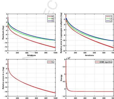
001 givesagoodconvergencespeedaseachpairofcurvesin

Fig. 2

(a) and(b)decreasetozerowithverysimilarspeed.Inaddition,

Fig. 2

(d)showsthatthenumericalenergyoftheTWSOmodel

(2.3)

has reachedtoasteadystate afteronlyafewiterations.

Fig. 2

shows theplotsforarealinpaintingexamplein

Fig. 7

.

TheresidualsRk_i

(

i

=

1

,

2

,

3

)

aredefinedas

Rk₁

,

Rk₂

,

Rk₃

=

1

|

|

˜

u

k

_{− ˜}

_uk

L1

,

1

|

|

V

k

_{− ∇}

2_uk

L1

,

1

|

|

W

k

₋

_TVk

L1

,

(5.1)

where

·

L1 denotes the L1-norm on the image domain

.

The relative errors of the augmented Lagrangian multipliers Lk

i

(

i

=

1

,

2

,

3

)

aredefinedas

Lk₁

,

Lk₂

,

Lk₃

=

||

sk

₋

_sk−1

_||

L1

||

sk−1

_||

L1

,

||

d

k

₋

_dk−1

_||

L1

||

dk−1

_||

L1

,

||

b

k

₋

_bk−1

_||

L1

||

bk−1

_||

L1

.

(5.2)

Therelativeerrorsofuaredefinedas

Rk_u

=

||

u

k

₋

_uk−1

_||

L1

||

uk−1

_||

L1

.

(5.3)

In summary, there are only two built-in parameters

ρ

and

C

that need to be adjusted forinpainting different images(see

Ta-ble 1fortheir selections).Consequently,the proposed TWSOisa

1 67

2 68

3 69

4 70

5 71

6 72

7 73

8 74

9 75

10 76

11 77

12 78

13 79

14 80

15 81

16 82

17 83

18 84

19 85

20 86

21 87

22 88

23 89

24 90

25 91

26 92

27 93

28 94

29 95

30 96

31 97

32 98

33 99

34 100

35 101

36 102

37 103

38 104

39 105

40 106

41 107

42 108

43 109

44 110

45 111

46 112

47 113

48 114

49 115

50 116

51 117

52 118

53 119

54 120

55 121

56 122

57 123

58 124

59 125

60 126

61 127

62 128

63 129

64 130

65 131

[image:6.612.106.477.58.369.2]

66 132

Fig. 2.Plots of the residuals (5.1), the relative errors of the Lagrangian multipliers (5.2), the relative errors of the function uin (5.3), and the energy of the proposed model (2.3)against number of iterations for the real inpainting example in Fig. 7.

[image:6.612.105.477.398.722.2]

1 67

2 68

3 69

4 70

5 71

6 72

7 73

8 74

9 75

10 76

11 77

12 78

13 79

14 80

15 81

16 82

17 83

18 84

19 85

20 86

21 87

22 88

23 89

24 90

25 91

26 92

27 93

28 94

29 95

30 96

31 97

32 98

33 99

34 100

35 101

36 102

37 103

38 104

39 105

40 106

41 107

42 108

43 109

44 110

45 111

46 112

47 113

48 114

49 115

50 116

51 117

52 118

53 119

54 120

55 121

56 122

57 123

58 124

59 125

60 126

61 127

62 128

63 129

64 130

65 131

66 132

Table 1

Parameters used in the TWSO model for the examples in Figs. 4–7and Figs. 9–10.

Parameter Fig. 4 Fig. 5 Fig. 6 Fig. 7 Fig. 9 Fig. 10

1st, 2nd columns 3rd, 4th columns 5th, 6th columns All rows

ρ 10 10 10 10 10 5 1 1

σ 1 1 1 1 1 1 1 1

γ 0.01 0.01 0.01 0.01 0.01 0.01 – –

C/C 10 1 5 1 1 1 5 5

η 100 100 100 100 100 100 0.04 0.05

θ1 0.01 0.01 0.01 0.01 0.01 0.01 5 5

θ2 0.01 0.01 0.01 0.01 0.01 0.01 5 5

θ3 0.001 0.001 0.001 0.001 0.001 0.001 10 10

Fig. 4.Performance comparison of the SOTV and TWSO models on some degraded images. The red regions in the first row are inpainting domains. The second and third rows show the corresponding inpainting results by the SOTV and the TWSO models, respectively. (For interpretation of the references to colour in this figure legend, the reader is referred to the web version of this article.)

Fig. 5.Test on a black stripe with different geometries. (a): Images with red inpaint-ing regions. The last three inpaintinpaint-ing gaps have the same width but with different geometry; (b–f): results of TV, SOTV, TGV, Euler’s elastica, and TWSO, respectively. (For interpretation of the references to colour in this figure legend, the reader is referred to the web version of this article.)

For image denoising, there are 7 parameters in the TWSO

model:

ρ

and

σ

in (2.5), the contrastparameter C in

(2.9)

, and

η

,

θ

1,

θ

2 and

θ

3 in (4.4).Each parameter plays a similar role as

its counterpart in the inpainting model. However, in contrast to

inpainting,

ρ

hereshouldbesmallbecausewedonotneedto

con-nectgaps forimagedenoising. We havealsofound that

σ

=

1 is

sufficientforthecasesconsideredinthispaper.C determineshow

muchanisotropy theTWSO modelwillbringto theresulting

im-age.We illustrate theeffect ofthisparameter usingthe example

in Fig. 10.The regularisation parameter

η

should be smallwhen

image noise level ishigh. The three penalty parameters are cho-senbasedonthequantitiesdefinedin

(5.1)

,

(5.2)

and

(5.3)

.

Fig. 3

showsthatusing

θ

1

=

5,

θ

2

=

5 and

θ

3

=

10 leadstofast conver-gencespeedforthesyntheticimagein

Fig. 9

andthesevaluesare usedfortherestofimagedenoisingexamples.Finally,the param-etersselectedaregiveninthelasttwocolumnsin

Table 1

.

5.2. Imageinpainting

In thissection we test the capability of the TWSO model for

image inpainting andcompare itwithseveral state-of-the-art in-paintingmethodssuchastheTV

[36]

,TGV

[37]

,SOTV

[2,22]

,and Euler’selastica

[21,38]

models.We denotethe inpainting domain asD inthefollowingexperiments.Theregion

inequation

(2.3)

is

\

D.Weuse p

=

2 forallexamplesinimageinpainting.

Fig. 4illustratestheimportanceofthetensorTintheproposed

TWSOmodel.Thedamaged imagesoverlaid withthered

inpaint-ingdomainsareshowninthefirstrow.Secondrowandthirdrow

show that theTWSO performs muchbetter thanSOTV.SOTV

in-troducesblurring tothe inpainted regions, whilst TWSOrecovers theseshapesverywellwithoutcausingmuchblurring.Inaddition to the capability ofinpainting large gaps, the TWSO interpolates

smoothly along the level curves of the image in the inpainting

domain,indicatingtheeffectivenessoftensorinTWSOfor inpaint-ing.

In

Fig. 5

,we show howdifferent geometriesof theinpainting region affectthe results by different methods. Column (b) illus-tratesthatTVperformssatisfactorilyiftheinpaintingareaisthin. However,itfailsinimagesthatcontainlargegaps.Column(c) indi-catesthattheinpaintingresultbySOTVdependsonthegeometry oftheinpaintingregion.Itisabletoinpaintlargegapsbutatthe

1 67

2 68

3 69

4 70

5 71

6 72

7 73

8 74

9 75

10 76

11 77

12 78

13 79

14 80

15 81

16 82

17 83

18 84

19 85

20 86

21 87

22 88

23 89

24 90

25 91

26 92

27 93

28 94

29 95

30 96

31 97

32 98

33 99

34 100

35 101

36 102

37 103

38 104

39 105

40 106

41 107

42 108

43 109

44 110

45 111

46 112

47 113

48 114

49 115

50 116

51 117

52 118

53 119

54 120

55 121

56 122

57 123

58 124

59 125

60 126

61 127

62 128

63 129

64 130

65 131

66 132

Fig. 7.Real example inpainting. “Cornelia, mother of the Gracchi” by J. Suvee (Louvre). From left to right are degraded image, inpainting results of TV, SOTV, TGV, Euler’s elastica, and TWSO, respectively; Second row shows the local magnification of the corresponding results in the first row.

Table 2

Comparison of PSNR and SSIM of different methods inFigs. 5–7.

PSNR test SSIM value

Figure # Fig. 5 Fig. 6 Fig. 7 Fig. 5 Fig. 6 Fig. 7

1st_{row 2}nd_{row 3}rd_{row 4}th_{row 1st row 2nd row 3rd row 4th row}

Degraded 18.5316 12.1754 11.9285 11.6201 8.1022 14.9359 0.9418 0.9220 0.8778 0.8085 0.5541 0.8589

TV Inf 12.7107 12.7107 12.7107 14.4360 35.7886 1.0000 0.9230 0.9230 0.9230 0.6028 0.9936

SOTV 28.7742 14.1931 18.5122 12.8831 14.9846 35.6840 0.9739 0.9289 0.9165 0.8118 0.6911 0.9951

TGV 43.9326 12.7446 12.7551 13.4604 14.0600 36.0854 0.9995 0.9232 0.9233 0.8167 0.6014 0.9941

Euler’s elastica 70.2979 54.0630 51.0182 13.0504 14.8741 34.3064 1.0000 0.9946 0.9982 0.8871 0.6594 0.9878

TWSO Inf Inf Inf 43.3365 27.7241 41.1400 1.0000 1.0000 1.0000 0.9992 0.9689 0.9976

Table 3

Mean and standard deviation (SD) of PSNR and SSIM calculated using 5 different methods for image inpainting over 100 images from the Berkeley database BSDS500 with 4 different random masks.

PSNR value (Mean±SD) SSIM value (Mean±SD)

Missing 40% 60% 80% 90% 40% 60% 80% 90%

Degraded 9.020±0.4208 7.250±0.4200 6.010±0.4248 5.490±0.4245 0.05±0.0302 0.03±0.0158 0.01±0.0065 0.007±0.003 TV 31.99±3.5473 28.68±3.3217 24.61±2.7248 20.94±2.2431 0.92±0.0251 0.84±0.0412 0.67±0.0638 0.48±0.0771 TGV 31.84±3.9221 28.70±3.8181 25.52±3.6559 23.32±3.5221 0.93±0.0310 0.87±0.0580 0.75±0.1023 0.64±0.1372 SOTV 32.43±4.9447 29.39±4.5756 26.38±4.2877 24.41±4.0720 0.94±0.0308 0.89±0.0531 0.80±0.0902 0.71±0.1204 Euler’s elastica 32.12±4.0617 29.21±3.9857 26.30±3.8194 24.34±3.6208 0.94±0.0288 0.88±0.0526 0.78±0.0901 0.69±0.1208 TWSO 34.33±3.4049 31.12±3.0650 27.66±3.6540 25.26±3.2437 0.95±0.0204 0.90±0.0456 0.82±0.0853 0.73±0.1061

costofintroducingblurring.Mathematically,TGVisacombination ofTVandSOTV,soitsresults,asshowninColumn(d),aresimilar

tothoseofTVandSOTV.TGVresultsalsoseemtodependonthe

geometryoftheinpaintingarea.ThelastcolumnshowsthatTWSO inpaintsthe imagesperfectlywithoutanyblurring andregardless localgeometry. TWSO isalso slightlybetter than Euler’selastica, whichhasproventobeveryeffectiveindealingwithlargergaps.

Wenow showan exampleofinpainting asmooth image with

large gaps. Fig. 6 showsthat all the methods, except the TWSO

model,fail ininpainting the largegaps inthe image. Thisis due to the fact that TWSO integrates the tensor T with its eigenval-uesdefinedin

(2.10)

, whichmakes itsuitable forrestoringlinear structures,asshowninthesecondrowof

Fig. 6

.

Fig. 7comparestheinpaintingofarealimagebyallthe

meth-ods.TheinpaintingresultoftheTVmodelseemstobemore satis-factorythanthoseofSOTVandTGV,thoughitproducespiecewise constantrestoration. Fromthesecond row,neitherTV norTGVis

able to connect the gaps on the cloth. SOTV reduces some gaps

but blurs the connecting region. Euler’s elastica performs better

than TV,SOTV andTGV, but nobetter than the proposed TWSO

model.

Table 2

showsthattheTWSO isthemostaccurateamong

allthemethodscomparedfortheexamplesin

Figs. 5–7

.

Finally,we evaluateTV, SOTV,TGV,Euler’s elasticaandTWSO

ontheBerkeleydatabaseBSDS500forimageinpainting.Weuse4

randommasks(i.e.40%,60%, 80% and90% pixelsaremissing)for

each ofthe100imagesrandomlyselectedfromthedatabase.The

performance ofeachmethodforeachmask ismeasuredinterms

of mean andstandard derivation ofPSNR and SSIM over all 100

images.Theresultsaredemonstratedinthefollowing

Table 3

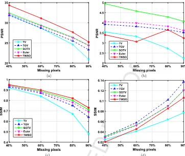
and

Fig. 8.Theaccuracyoftheinpaintingresultsobtainedbydifferent

methods decreasesasthepercentageofmissingpixelsregion be-comeslarger.ThehighestaveragedPSNRvaluesareagainachieved bytheTWSO,demonstratingitseffectivenessforimageinpainting.

5.3. Imagedenoising

FordenoisingimagescorruptedbyGaussiannoise,weuse p

=

2 in (2.3) andthe

in (2.3) is the same as the image domain

.WecomparetheproposedTWSOmodelwiththePerona–Malik

(PM)

[39]

,coherentenhancingdiffusion(CED)

[32]

,totalvariation (TV)

[40]

,second ordertotalvariation(SOTV)

[1,22,26]

,total gen-eralised variation (TGV) [30], and extended anisotropic diffusion model4 _(EAD)

_[11]

_{onbothsyntheticandrealimages.}

Fig. 9 showsthe denoisedresultson a syntheticimage (a)by

differentmethods.TheresultsbythePMandTVmodels,asshown in (c) and (e), have a jagged appearance (i.e. staircase artefact).

1 67

2 68

3 69

4 70

5 71

6 72

7 73

8 74

9 75

10 76

11 77

12 78

13 79

14 80

15 81

16 82

17 83

18 84

19 85

20 86

21 87

22 88

23 89

24 90

25 91

26 92

27 93

28 94

29 95

30 96

31 97

32 98

33 99

34 100

35 101

36 102

37 103

38 104

39 105

40 106

41 107

42 108

43 109

44 110

45 111

46 112

47 113

48 114

49 115

50 116

51 117

52 118

53 119

54 120

55 121

56 122

57 123

58 124

59 125

60 126

61 127

62 128

63 129

64 130

65 131

[image:9.612.124.486.54.358.2]

66 132

[image:9.612.46.556.392.519.2]

Fig. 8.Plots of mean and standard derivation in Table 3obtained by 5 different methods over 100 images from the Berkeley database BSDS500 with 4 different random masks. (a) and (b): mean and standard derivation plots of PSNR; (c) and (d): mean and standard derivation plots of SSIM.

Fig. 9.Denoising results of a synthetic test image. (a) Clean data; (b) Image corrupted by 0.02 variance Gaussian noise; (c–i): Results of PM, CED, TV, SOTV, TGV, EAD, and TWSO, respectively. Second row shows the isosurface rendering of the corresponding results above.

However, the scale-space-based PM model shows much stronger

staircaseeffectthantheenergy-basedvariationalTVmodelfor de-noisingpiecewisesmoothimages.Duetotheanisotropy,theresult (d)by theCEDmethoddisplays strongdirectional characteristics.

Due to the high order derivatives involved, the SOTV, TGV and

TWSOmodelscanreducethestaircaseartefact.However,because

the SOTV imposes too much regularity on the image, it smears

the sharpedges of theobjects in(f). Better results are obtained

by the TGV, EAD and TWSO models, which show no staircase

andblurringeffects,though TGV leavessome noise nearthe

dis-continuities andEAD over-smoothsimage edges, asshownin (g)

and (h).

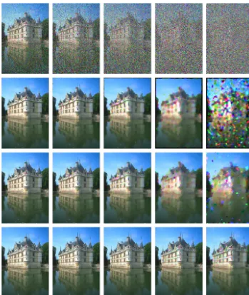
Fig. 10presentsthedenoisedresultsonarealimage(a)by

dif-ferentmethods.BoththeCEDandtheproposedTWSOmodelsuse

the anisotropic diffusion tensor T. CED distorts the image while

TWSOdoesnot. Thereasonforthisisthat TWSOusesthe

eigen-valuesofTdefinedin

(2.9)

,whichhastwoadvantages:i)itallows ustocontrolthedegreeoftheanisotropyofTWSO.Ifthecontrast

parameterCin

(2.9)

goestoinfinity,theTWSOmodeldegenerates to theisotropic SOTV model.The larger C is,the lessanisotropy

TWSO has.The eigenvalues (2.10) used in CED however are not

able to adjust theanisotropy; ii)it can determine ifthere exists diffusion inTWSO along the directionparallel to the image gra-dient. Thediffusionhaltsalongtheimage gradientdirectionif

λ

1 in

(2.9)

issmallandencouragedif

λ

1 islarge.Bychoosinga suit-ableC,

(2.9)

allowsTWSO todiffusethenoisealongobjectedges andprohibitthediffusionacrossedges.Theeigenvalue

λ

1 usedin

(2.10) howeverremains small(i.e.

λ

1

1) all the time, meaning

that the diffusionalong image gradient inCEDis always prohib-ited.CEDthusonlypreferstheorientationthatisperpendicularto theimagegradient,whichexplainswhyCEDdistortstheimage.

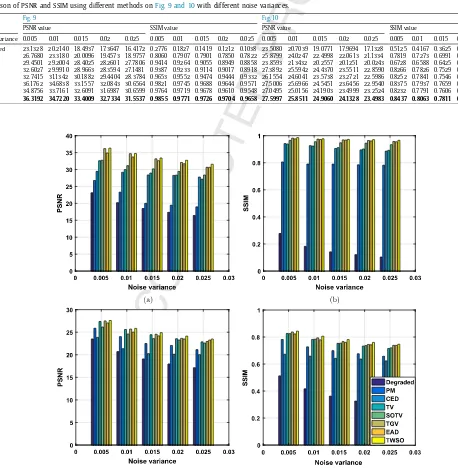
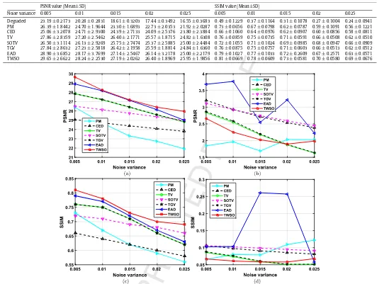
In addition to qualitative evaluation of different methods in

Fig. 9 and 10, we also calculate the PSNR and SSIM values for

thesemethodsandshowthemin

Table 4

and

Fig. 11

.These

met-ricsshowthatthePDE-basedmethods(i.e.PMandCED)perform

1 67

2 68

3 69

4 70

5 71

6 72

7 73

8 74

9 75

10 76

11 77

12 78

13 79

14 80

15 81

16 82

17 83

18 84

19 85

20 86

21 87

22 88

23 89

24 90

25 91

26 92

27 93

28 94

29 95

30 96

31 97

32 98

33 99

34 100

35 101

36 102

37 103

38 104

39 105

40 106

41 107

42 108

43 109

44 110

45 111

46 112

47 113

48 114

49 115

50 116

51 117

52 118

53 119

54 120

55 121

56 122

57 123

58 124

59 125

60 126

61 127

62 128

63 129

64 130

65 131

[image:10.612.37.549.58.186.2]

66 132

Fig. 10.Noise reduction results of a real test image. (a) Clean data; (b) Noisy data corrupted by 0.015 variance Gaussian noise; (c–i): Results of PM, CED, TV, SOTV, TGV, EAD, and TWSO, respectively. The second row shows local magnification of the corresponding results in the first row.

Table 4

Comparison of PSNR and SSIM using different methods on Fig. 9 and 10with different noise variances.

Fig. 9 Fig. 10

PSNR value SSIM value PSNR value SSIM value

Noise variance 0.005 0.01 0.015 0.02 0.025 0.005 0.01 0.015 0.02 0.025 0.005 0.01 0.015 0.02 0.025 0.005 0.01 0.015 0.02 0.025

Degraded 23.1328 20.2140 18.4937 17.3647 16.4172 0.2776 0.1827 0.1419 0.1212 0.1038 23.5080 20.7039 19.0771 17.9694 17.1328 0.5125 0.4167 0.3625 0.3261 0.3009 PM 26.7680 23.3180 20.0096 19.4573 18.9757 0.8060 0.7907 0.7901 0.7850 0.7822 25.8799 24.0247 22.4998 22.0613 21.1334 0.7819 0.7273 0.6991 0.6760 0.6579 CED 29.4501 29.2004 28.4025 28.2601 27.7806 0.9414 0.9264 0.9055 0.8949 0.8858 23.8593 21.3432 20.2557 20.1251 20.0243 0.6728 0.6588 0.6425 0.6375 0.6233 TV 32.6027 29.9910 28.9663 28.3594 27.1481 0.9387 0.9233 0.9114 0.9017 0.8918 27.3892 25.5942 24.4370 23.5511 22.8590 0.8266 0.7826 0.7529 0.7331 0.7149 SOTV 32.7415 31.1342 30.1882 29.4404 28.3784 0.9653 0.9552 0.9474 0.9444 0.9332 26.1554 24.6041 23.5738 23.2721 22.5986 0.8252 0.7841 0.7546 0.7367 0.7201 TGV 36.1762 34.6838 33.1557 32.0843 30.6564 0.9821 0.9745 0.9688 0.9644 0.9571 27.5006 25.6966 24.5451 23.6456 22.9540 0.8375 0.7937 0.7659 0.7456 0.7386 EAD 34.8756 33.7161 32.6091 31.6987 30.6599 0.9764 0.9719 0.9678 0.9610 0.9548 27.0495 25.0156 24.1903 23.4999 23.2524 0.8232 0.7791 0.7606 0.7424 0.7382 TWSO 36.3192 34.7220 33.4009 32.7334 31.5537 0.9855 0.9771 0.9726 0.9704 0.9658 27.5997 25.8511 24.9060 24.1328 23.4983 0.8437 0.8063 0.7811 0.7603 0.7467

[image:10.612.58.516.252.720.2]