Determining the halo mass scale where galaxies lose their gas

Determining the Halo Mass Scale Where Galaxies Lose Their Gas

Gregory Rudnick1,15 , Pascale Jablonka2,14, John Moustakas3, Alfonso Aragón-Salamanca4, Dennis Zaritsky5 , Yara L. Jaffé6,7 , Gabriella De Lucia8, Vandana Desai9 , Claire Halliday10, Dennis Just5,11 , Bo Milvang-Jensen12, and

Bianca Poggianti13 1

The University of Kansas, Department of Physics and Astronomy, Malott Room 1082, 1251 Wescoe Hall Drive, Lawrence, KS, 66045, USA;grudnick@ku.edu

2

Institut de Physique, Laboratoire d’astrophysique, Ecole Polytechnique Fédérale de Lausanne(EPFL), Observatoire de Sauverny, CH-1290 Versoix, Switzerland

3

Department of Physics & Astronomy, Siena College, 515 Loudon Road, Loudonville, NY 12211, USA

4_{School of Physics and Astronomy, The University of Nottingham, University Park, Nottingham NG7 2RD, UK} 5

University of Arizona, 933 N. Cherry Ave, Tucson, AZ 85721, USA

6

Department of Astronomy, Universidad de Concepción, Casilla 160-C, Concepción, Chile

7

European Southern Observatory, Alonso de Cordova 3107, Vitacura, Santiago, Chile

8

INAF-Osservatorio Astronomico di Trieste, Via Tiepolo 11, I-34131 Trieste, Italy

9

Spitzer Science Center, California Institute of Technology, MS 220-6, Pasadena, CA 91125, USA

10

23, rue d’Yerres, F-91230 Montgeron, France

11

Department of Astronomy & Astrophysics, University of Toronto, 50 St George Street, Toronto, ON M5S 3H4, Canada

12

Dark Cosmology Centre, Niels Bohr Institute, University of Copenhagen, Juliane Maries Vej 30, DK-2100 Copenhagen, Denmark

13

INAF-Osservatorio Astronomico di Padova, Vicolo dell Osservatorio 5, I-35122 Padova, Italy

14

GEPI, Observatoire de Paris, CNRS, Université Paris Diderot, F-92125 Meudon Cedex, France Received 2016 June 24; revised 2017 August 4; accepted 2017 August 4; published 2017 November 30

Abstract

A major question in galaxy formation is how the gas supply that fuels activity in galaxies is modulated by their environment. We use spectroscopy of a set of well-characterized clusters and groups at 0.4<z<0.8 from the ESO Distant Cluster Survey and compare it to identically selected field galaxies. Our spectroscopy allows us to isolate galaxies that are dominated by old stellar populations. Here we study a stellar-mass-limited sample

(log(M_* M)>10.4)of these old galaxies with weak[OII]emission. We use line ratios and compare to studies of local early-type galaxies to conclude that this gas is likely excited by post-AGB stars and hence represents a diffuse gas component in the galaxies. For cluster and group galaxies the fraction with EW([OII])>5Å is f_[O II]=

-+

0.08 0.020.03 and f[O II]=0.06-+0.040.07, respectively. For field galaxies wefind f[O II]=0.27-+0.060.07, representing a 2.8σ

difference between the [OII]fractions for old galaxies between the different environments. We conclude that a population of old galaxies in all environments has ionized gas that likely stems from stellar mass loss. In thefield galaxies also experience gas accretion from the cosmic web, and in groups and clusters these galaxies have had their gas accretion shut off by their environment. Additionally, galaxies with emission preferentially avoid the virialized region of the cluster in position–velocity space. We discuss the implications of our results, among which is that gas accretion shutoff is likely effective at group halo masses(log/>12.8)and that there are likely multiple gas removal processes happening in dense environments.

Key words:galaxies: evolution –galaxies: groups: general –galaxies: ISM

Supporting material:machine-readable table

1. Introduction

One of the longest-standing problems in galaxy evolution is how star formation in galaxies is quenched. We have known for over 50 yr that there is a significant population of galaxies with uniformly red colors that occupy a tight sequence in color and magnitude (e.g., de Vaucouleurs 1961; Visvanathan & Sandage1977). Couch et al.(1983), Butcher & Oemler(1984), and Bower et al.(1992a,1992b)interpreted this tight sequence as resulting from uniformly old stellar ages for these “red sequence” galaxies. The tight scatter in color of the red sequence in turn implies that galaxies must stay passive for extended periods (e.g., Aragon-Salamanca et al.1993; Bower et al. 1998; Kodama et al. 1998). Subsequently, it was demonstrated that the distribution of galaxy star formation rates

(SFRs) and star formation histories (SFHs) is approximately

bimodal, with galaxies either forming stars or being passive

(e.g., Strateva et al.2001; Kauffmann et al.2003), although this bimodality might be less pronounced for the most massive galaxies(e.g., Salim et al.2007). Lookback studies have shown that the amount of stellar mass in the star-forming population remains relatively constant at z<1.5, while the mass in the passive population increases over the same epoch (e.g., Bell et al. 2004; Blanton 2006; Brammer et al. 2011). This is as would be expected if star-forming galaxies were quenched and added to the passive population progressively over time. However, despite the ample evidence for galaxy quenching, it is not clear whether this quenching is rapid (e.g., Bell et al. 2004)or slow(e.g., Schawinski et al.2014).

At about the same time, it was also realized that the fraction of galaxies that are passive depends on environment. In the local rich clusters such as Coma, the passive population completely dominates(Terlevich et al. 2001), but even in less extreme environments it is clear that denser environments host a larger fraction of passive galaxies(Hogg et al.2004; Blanton & Moustakas 2009). One possible explanation for these observed correlations is that there are physical processes that © 2017. The American Astronomical Society. All rights reserved.

* _{Based on observations obtained at the European Southern Observatory using} the ESO Very Large Telescope on Cerro Paranal through ESO program 166. A-0162.

15

occur in dense environments that suppress star formation in galaxies. The color–density relation holds to at least z=2

(Cooper et al.2006; Gerke et al.2007; Cooper et al.2010; Peng et al. 2010; Quadri et al.2011), and if this is indicative of an active suppression of star formation in dense environments, it indicates that these processes may have been important over a majority of cosmic time. However, an alternate explanation for the SFR–density relation is that galaxies in dense environments are simply older than those in lower-density regions, presumably echoing an earlier formation epoch (e.g., Gao et al.2005; Tonnesen & Cen2015).

It is difficult to disentangle these two possibilities, and much work has been done to isolate the signatures of specific transformative processes. On the observational side, there is mounting evidence that whatever shuts off star formation in galaxies entering dense environments must precede a transfor-mation in the morphology. For example, the rapid buildup in the red sequence luminosity function atz<0.8(De Lucia et al.

2004,2007; Tanaka et al.2005; Stott et al.2007; Gilbank et al.

2008; Rudnick et al. 2012; but see also Andreon 2008;

Crawford et al.2009; De Propris et al.2013)seems to precede the buildup in the S0 population that becomes significant at

z<0.5 (Desai et al. 2007a). This sequencing of gas and morphological processes is also supported by the lack of blue S0 galaxies(Jaffé et al. 2011)in clusters and the lack of UV emission in S0s found in a merger of galaxy groups(Just et al. 2011), both of which indicate that galaxies change their morphology after their star formation is suppressed. Indeed, in Gallazzi et al.(2009)and Wolf et al.(2009)it was found that there is a population of spiral galaxies in the A901/902 supercluster that have spiral morphology but suppressed star formation. A similar population of galaxies is even found in intermediate-redshift clusters (Cantale et al.2016) and in the field(Bundy et al.2010).

The quenching of star formation without a commensurate change in morphology argues strongly for processes that suppress star formation by the depletion of gas in galaxies. There are multiple theoretical mechanisms for the gas to be affected in galaxies. Strangulation or starvation,first proposed by Larson et al.(1980), is now understood to encompass the broad family of processes in which galaxies decouple from the gas that flows into them from the intergalactic medium(IGM)and thus use up their internal gas supply on an extended timescale of a few Gyr. This process seems to match the observed increase with time in the quenched fraction of galaxies in dense environments

(e.g., McGee et al. 2011; De Lucia et al. 2012; Taranu et al.

2014; Haines et al.2015). This mechanism should be effective

all the way down to at least group scales, as satellite galaxies in those halos should be decoupled from their gasflows(Kawata & Mulchaey2008). Indeed, observations of galaxies in groupsfind them to be HIdeficient with respect to matched galaxies in the field(Catinella et al.2013).

A modification of the starvation scenario discussed by various authors has been the role of winds in speeding up the depletion of gas once accretion is shut off (e.g., Weinmann et al. 2006; Wang et al. 2007). These winds are known to be ubiquitous in star-forming galaxies (e.g., Weiner et al.2009; Rubin et al.2010,2014), but with an uncertain mass loading. Recently, McGee et al. (2014) found that winds with reason-able mass-loading factors could, when coupled with a long-delay time upon becoming a satellite (Wetzel et al. 2013), explain both the long timescales for transformation to happen

for infalling satellite galaxies and the rapid shutoff in star formation once the delay time has passed. This wind-driven consumption was termed by McGee et al. (2014) as “ over-consumption” and is able to explain the observed weak dependence of the SFR of star-forming galaxies on environ-ment, which implies that star formation must be shut off quickly(Peng et al.2010; McGee et al.2011).

An alternate process for the suppression of star formation is the stripping of the cold gas via ram pressure effects(Gunn & Gott 1972), which results from a galaxy passing through the dense intracluster medium (ICM). Theoretical investigations have shown that this process can remove significant amounts of both diffuse and cold gas from within the optical radius of galaxies in rich cluster environments (Quilis et al. 2000; Roediger & Brüggen 2007, 2008; Tonnesen & Bryan 2009). Observational investigations have shown both dramatic strip-ping of the gas content of galaxies in cluster environments

(Kenney & Koopmann1999; Kenney et al.2004; Cortese et al.

2011; Pappalardo et al. 2012; Boselli et al. 2014; Fumagalli

et al.2014; Jáchym et al.2014; Jaffé et al.2015)and statistical evidence from rotation curve asymmetries in cluster galaxies with normal morphology that ram pressure stripping is likely important in those environments(Bösch et al.2013).

Contrary to common conceptions, ram pressure stripping need not be fast (∼100 Myr), as the fast timescales inferred from theoretical investigations (Quilis et al. 2000) are only valid if galaxies are inserted at high speeds into a dense ICM. Galaxies falling into the cluster from larger radii instead will experience ram pressure stripping on a longer timescale more akin to a crossing time, as the pressure builds up during the infall process as a result of the increasing velocity and ICM density. The actual modification to the gas of a galaxy suffering ram pressure stripping depends sensitively on the orbit of the galaxy at infall, as galaxies with different orbits will spend different times in the region of the cluster with the highest ram pressure(e.g., Brüggen & De Lucia2008; Jaffé et al. 2015).

Despite much work on understanding the effects of environ-ment on galaxy gas, the relative roles of starvation and ram pressure stripping have proven difficult to disentangle, as the timescales may not be as different as previously thought, and because few observations trace a large dynamic range in density and contain a significant number of high-density systems. It is clear that there is a population of star-forming galaxies in clusters that exhibit slightly suppressed SFRs (Vulcani et al.

2010; Haines et al.2013), which may indicate a slow quenching

process. However, there is still a significant degree of tension between the quenching timescales inferred by the above physical mechanisms and the very long quenching timescales needed to reproduce the evolution in the galaxy passive fractions over cosmic time(McGee et al. 2011; De Lucia et al.2012; Wetzel et al.2013). It is therefore necessary to examine both of these processes in more detail and to determine which of the processes are required by the observations, which are ruled out, which are merely allowed, and over what halo mass ranges these different conclusions hold.

An additional question that needs to be resolved is how to keep dead(or passive)galaxies dead. Galaxies replenish their gas through mass loss, with a Chabrier (2003) or Kroupa

(2001)initial mass function(IMF)returning∼40%(50%)of a simple stellar population’s stellar mass to gas within 1

(13)Gyr. It is not clear how to keep that gas from forming stars. This gas is observed to exist in local galaxies, as studies

have shown that emission lines from ionized gas (e.g., [OII], Hα)in passive galaxies are common, may be supplied by mass loss, and may be predominantly heated by existing stellar populations (Sarzi et al.2006, 2010; Yan et al. 2006; Yan & Blanton2012; Singh et al.2013; Belfiore et al.2016). There are some indications as well from integral field spectroscopic identification of distinct kinematic components that this gas can be supplied by external accretion and that external accretion is not a significant supply of replenished gas in Virgo Cluster galaxies(Davis et al.2011). Despite the insight granted by their 3D (spatial+kinematic)data, these local studies are limited to only a single cluster and do not adequately probe the group environment. Thus, the effect of environment on this supply of gas is still not well understood.

To better understand the mechanisms through which the gas supply is modulated in galaxies, we mustfirstfind a population of galaxies that have a specific signature of gas depletion/ removal. We must then examine how this population changes as a function of halo mass, across a broad range of stellar mass, and also how the population changes as a function of position and velocity with respect to the host halo. That is the purpose of this paper.

Studying galaxies in intermediate-redshift clusters is a promising place to examine the gas mechanisms at play when clusters were growing rapidly and when galaxy quenching was proceeding at a rapid pace. While studies in the local universe, for example, using Sloan Digital Sky Survey(SDSS)data, have a plethora of line indices to characterize the gas, SDSS is subject to significant aperture biases (e.g., Brinchmann et al.

2004; Labbé et al. 2007)that complicate the interpretation of

the line emission in terms of the global properties of the galaxies. On the other hand, slit spectra of intermediate-redshift galaxies capture a majority of the galaxy light, making them more straightforward probes of integrated galaxy properties. While integral field spectroscopic surveys such as SAURON

(de Zeeuw et al.2002), ATLAS3D(Cappellari et al.2011), and CALIFA(Singh et al.2013)probe spatially integrated emission processes in the nearby universe, and especially the case of emission in passive galaxies(e.g., Sarzi et al.2006), they only contained one dense environment, i.e., the Virgo Cluster, making it difficult for those surveys to draw significant conclusions about the effect of environment. New integral field surveys such as SDSS-Manga (Bundy et al. 2015) and SAMI(Bryant et al.2015)are starting to probe environmental dependence of gas properties. However, there is now evidence that the quenching mechanism may have been different at higher redshift, due to the different density of the ICM and the higher gas fractions of galaxies (e.g., Balogh et al. 2016). Therefore, if we want to understand gas accretion shutoff processes at intermediate redshift, which are responsible for the quenching of many passive galaxies in today’s clusters, it is best to probe intermediate-redshift galaxies directly.

We employ spectroscopic observations of a large sample of field, group, and cluster galaxies at 0.4<z<0.8 collected as part of the ESO Distant Cluster Survey(EDisCS; White et al. 2005). Our spectroscopic observations of Hδabs and Hγabs

Balmer absorption lines, the 4000Å break, and various emission lines allow us to determine the recent SFH and current SFR of our galaxies in a stellar-mass-selected sample

(Barger et al. 1996; Rudnick et al. 2000; Kauffmann et al. 2003). We isolate a population of galaxies dominated by older stellar populations yet having emission lines and then

determine what their prevalence and characteristics tell us about gas stripping and starvation properties in dense environments. We examine many possibilities to explain the observed results and conclude on what possibilities are required by the observations and which are merely allowed.

The outline of our paper is as follows. In Section 2 we discuss our sample, photometric and spectroscopic measure-ments, and stellar mass determination. In Section3we discuss our use of spectral indices to isolate galaxies with different relative stellar ages and analyze their broadband spectral properties. In Section 4 we present the environmental dependence of our older galaxies with emission lines, including their distribution in velocity and position in our clusters. In Section5we discuss the origin of the observed environmental differences and use a comprehensive decision tree to decide on what is allowed and required by our observations. We summarize and conclude in Section6.

Throughout we assume“concordance”Λ-dominated cosmology withΩM=0.3,ΩΛ=0.7, andH0=70h70km s−1Mpc−1unless

explicitly stated otherwise. All magnitudes are quoted in the AB system(Oke1974).

2. Data

2.1. Sample Definition, Photometry, and Morphologies

Our data are infields observed by the EDisCS. Eachfield was selected to have a primary optically selected cluster. The exact selection of the parent EDisCS fields and the main clusters is described in detail in White et al.(2005). In some fields there are additional clusters and groups serendipitously discovered along the line of sight. Eachfield was observed with

BVIKs,BVIJKs, orVRIJKsphotometry depending on the initial redshift estimate. The optical data were obtained with VLT/ FORS2 and the near-IR data with NTT/SOFI. Vega-to-AB magnitude conversions were computed by integrating the spectrum of Vega over ourfilter curves.

As part of EDisCS we have obtained 30–50 spectra of members per main cluster and significant numbers in the projected groups and clusters along the line of sight, as well as manyfield galaxies at similar redshifts to the main structures

(Halliday et al.2004; Milvang-Jensen et al.2008). For objects that were observed multiple times, we replaced the multiple occurrences with a single measurement that is the average of the individual measurements.

We restrict our sample of groups andfield galaxies to those withinΔz=±0.2 of the main cluster redshift. It was shown in Halliday et al.(2004)and Milvang-Jensen et al.(2008)that the EDisCS spectroscopic target selection, which combined an

I-band magnitude cut and loose photometric redshift cuts(Pelló et al. 2009), missed an estimated 3% of the galaxies at the targeted cluster redshift compared to a strictly I-band-selected sample. Our spectroscopy withinΔz=±0.2 of the main cluster redshift is therefore unbiased. Following Poggianti et al.(2009), we classify clusters as those systems with a velocity dispersion

σ>400 km s−1 and groups as those with at least eight spectroscopic members and 160 km s−1<σ„400 km s−1. We further require our systems to have adequate exposures in all EDisCS bands to allow for the computation of stellar masses

therefore their stellar masses could not be computed robustly because our observations did not probe to red rest-frame optical wavelengths. The properties of our sample of structures are listed in Table1.

As galaxies evolve with redshift, it is important to control for differences in the redshift distribution of the galaxy samples in different environments. We test for this by comparing the redshift distributions for thefinal sample of galaxies in each of our three subsamples(cluster, group, andfield; see Section3.1 for final sample size). The median and 68% limits of the redshift distribution for the three samples are zmed,clust=

-+

0.60 0.14 0.19

, zmed,group=0.58-+0.18 0.15

, and zmed,field=0.63-+0.14 0.13

. Therefore, the distributions for all samples are identical, and our results will not be affected by different redshift distributions.

Using the velocity dispersion and redshift, we derive the halo mass for our structures using Equation (10) from Finn et al.

(2005). Our clusters occupy the halo mass range of 1013.8–1015.2 , and our groups correspond to 1012.8_–1013.8_{. It is}

important to note that the halo masses and velocity dispersions for our groups, especially the poorer groups, are quite uncertain. Membership in these structures is based on a 3σ cut in the velocity dispersion of the system, where σ is computed

iteratively using the biweight scale estimator (Beers et al.

1990; Halliday et al.2004; Milvang-Jensen et al.2008). In this

paper we only study the spectroscopic sample of galaxies. Our “field” sample consists of truefield galaxies in the sense that they do not belong to any structure withσ>160 km s−1.

Rest-frame luminosities were derived for each galaxy from the full spectral energy distribution using the technique described in Rudnick et al. (2009) and adopting the spectro-scopic redshift.16

We use visual morphologies derived from Hubble Space Telescope (HST)F814W imaging of 10 of the EDisCS fields

(Desai et al.2007b). This observed filter corresponds to rest-frameB- or V-band imaging of our systems depending on the redshift of the sample. The morphologies were derived by visual classifications by multiple team members (Desai et al.

2007b). The fields with HST morphology contain 11 of our

sample clusters andfive of our groups.

2.2. Stellar Masses

Stellar masses were derived using the iSEDfit code presented in Moustakas et al. (2013). In brief summary, we fit the observed photometry using a Bayesian technique that assumes exponentially declining or constant SFHs with superimposed random bursts. We use the Flexible Stellar Population Synthesis (FSPS) library from Conroy et al. (2009) and Conroy & Gunn (2010) with a Chabrier (2003) IMF and a Charlot & Fall(2000)attenuation curve. The IMF extends from 0.1 to 100. The masses derived with the FSPS library are less than 0.1dex different than when using the Bruzual & Charlot (2003) library. Our choice of attenuation curve also results in a difference in the masses of less than 0.1dex when compared to the Calzetti et al.(2000) curve. The inclusion of bursts in the SFH as opposed to a smooth SFH results in a difference of less than 0.1dex for most galaxies, with up to an 0.3dex difference for individual objects.

2.3. Spectral Indices

Much of our analysis relies on the ability to measure absorption features and weak emission lines from our spectra. The EDisCs spectra are well calibrated (Halliday et al. 2004; Milvang-Jensen et al.2008)and also allow the computation of line ratios. As we demonstrate in Section3.2.1, the indices we employ are far less susceptible to reddening than rest-frame optical colors and give a more clear mapping from the indices to an SFH. Specifically, we are interested in the age-sensitive Balmer absorption (Hδabs and Hγabs) and 4000Å break

(Dn(4000)) stellar continuum features, as well as the strong nebular emission lines[OII]λ3727,[OIII]λλ4959, 5007, and Hβ. The Dn(4000) index, first introduced by Balogh et al.

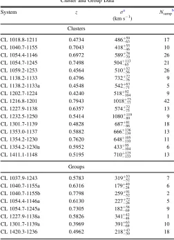
(1999), has a shorter-wavelength baseline than the traditionalD (4000) (Bruzual1983)and is therefore less susceptible to dust extinction. Our desire to separate out the emission and absorption components presents complications, as the emission lines can fill in the absorption features, and because the emission-line Table 1

Cluster and Group Data

System z σa Nsamp

b

(km s−1) Clusters

CL 1018.8-1211 0.4734 486-+6359 17

CL 1040.7-1155 0.7043 418-+4655 10

CL 1054.4-1146 0.6972 589-+7078 26

CL 1054.7-1245 0.7498 504-+65113 21

CL 1059.2-1253 0.4564 510-+5652 26

CL 1138.2-1133 0.4796 732-+7672 9

CL 1138.2-1133a 0.4548 542-+7163 5

CL 1202.7-1224 0.4240 518-+10492 9

CL 1216.8-1201 0.7943 1018-+7773 42

CL 1227.9-1138 0.6357 574-+7572 13

CL 1232.5-1250 0.5414 1080-+89119 9

CL 1301.7-1139 0.4828 687-+8681 18

CL 1353.0-1137 0.5882 666-+139136 13

CL 1354.2-1230 0.7620 648-+110105 11

CL 1354.2-1230a 0.5952 433-+10495 6

CL 1411.1-1148 0.5195 710-+133125 13

Groups

CL 1037.9-1243 0.5783 319-+5253 7

CL 1040.7-1155a 0.6316 179-+2640 6

CL 1040.7-1155b 0.7798 259-+5291 2

CL 1054.4-1146a 0.6130 227-+2872 5

CL 1054.7-1245a 0.7305 182-+6958 9

CL 1227.9-1138a 0.5826 341-+4642 1

CL 1301.7-1139a 0.3969 391-+6963 10

CL 1420.3-1236 0.4962 218-+5043 18

Notes. a

This was computed using the full EDisCS member sample, which is larger than the sample used for the analysis in this paper.

b

The number of galaxies meeting our stellar mass and quality cuts.

16

Two of our systems, CL 1138.2-1133 and CL 1138.2-1133a, do not have observedB-band photometry and, withz=0.48 and 0.45, respectively, lie at redshifts slightly below that where the rest-frameUband is purely interpolated from our photometry (z=0.53). The extrapolation to rest-frame U band, however, is small, with a minimal effect on the actual colors. The rest-frame luminosities in this paper are illustrative only and are not crucial to any part of our analysis. We have verified that the color–mass distribution of these clusters is similar to that of the others and include them in our sample.

measurements are difficult in regions of the spectra with many absorption features(e.g., Rudnick et al.2000). We address these complications by decomposing the emission and absorption using the techniques described in detail in Moustakas et al. (2010, 2011). Briefly, we model the stellar continuum as a non-negative linear combination of simple population synthesis models of various ages. We mask out the spectra at the expected location of all emission lines and sky features andfit in an iterative process that optimizes for the object’s redshift and velocity dispersion. As part of this process, the residuals to this fit—which contain continuum residuals and emission lines—are fit to obtain emission-linefluxes. These emission-linefits are then subtracted from the observed spectra. We individually inspected every spectrum to verify the quality of thefit and the decomposition of the absorption and emission lines. Some of thefits were able to be improved by flagging parts of the spectrum with sky residuals. Nonetheless, we were forced to remove some galaxies with poor fits, most of which resulted from significant sky residuals being coincident with lines of interest. The results of this process are a set of emission-line measurements and a continuum spectrum that has been “cleaned”of emission. We have multiple Balmer lines in our spectra to independently constrain the absorption and emission, and our decomposition is therefore robust.

From these data products, we measure the equivalent width of the[OII],[OIII], and Balmer emission lines. These lines are used to measure the SFR and to diagnose the presence of active galactic nucleus (AGN)activity. We also measure EW(Hδabs)

and EW(Hγabs), as these lines are measures of the

luminosity-weighted mean age and are useful indicators of the presence of young and intermediate-age stellar populations. Specifically, we use the Lick continuum and line windows as defined in Worthey & Ottaviani (1997) and Trager et al. (1998) to measure the Balmer absorption EWs. We quantify the amount of Balmer absorption using the average of the EW(Hδabs)

and EW(Hγabs) and call this index áHdabsHgabsñ. All index

measurements are given in Table2.

3. Galaxy Selection

3.1. Stellar Mass Completeness

Galaxy properties depend strongly on stellar mass (e.g., Kauffmann et al. 2003) and environment (e.g., Kauffmann et al. 2004), and we must therefore control for the former in order to study trends in the latter. We do this by selecting galaxies above a stellar mass limit for which we are complete to galaxies of all stellar mass-to-light ratios M_å/L. We determine an empirical stellar mass limit following Marchesini et al.

(2009)and Moustakas et al.(2013). We take galaxies between 0.1 and 1.5 mag brighter than our observed magnitude limit at each redshift and scale the stellar masses to the observed magnitude limit. The upper mass limit that encompasses 95% of the scaled masses gives us an indication of the maximum mass for which we are complete. Essentially this takes the maximum stellar mass-to-light ratio from our data and assumes that it is indicative of that at the magnitude limit. As described in Marchesini et al.(2009), this technique has advantages over traditional methods that use maximally old and unreddened stellar populations(e.g., Dickinson et al.2003)in that it makes fewer assumptions and derives the maximum M_å/L directly from the data.

The EDisCS spectroscopic magnitude limit is I=22 for 0.4<z<0.6 clusters and I=23 for 0.6<z<0.8 clusters.

The fainter selection at high redshift offsets the increasing luminosity distance, and the same mass limit log

(/)>10.4 applies for all of our systems. In all of what follows we only consider galaxies above this limit. This results in a total of 163, 55, and 251field, group, and cluster galaxies, respectively. In the last column of Table1we indicate the number of galaxies in thisfinal sample that come from each cluster and group.

3.2. Isolating Galaxies Dominated by Old Stars

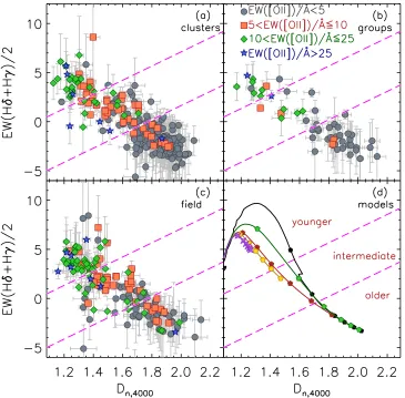
In Figure 1 we show the áHdabsHgabsñ strength versus

Dn(4000)for mass-selected cluster, group, andfield galaxies at 0.4<z<0.8, with the points coded by EW([OII]). It is clear that the galaxies in all environments follow a locus in this plot. As has been pointed out by many authors(e.g., Rudnick et al.

2000; Kauffmann et al.2003), this is a sequence of changing

luminosity-weighted age in galaxy stellar populations. Galaxies whose light is dominated by old stars appear in the lower right, with the fraction of young stars increasing to the upper left. We demonstrate this using model tracks in panel(d)of thefigure, derived from the Bruzual & Charlot (2003) stellar population synthesis code. These illustrative tracks represent a single stellar population (SSP) formed in a burst, a constant SFH model, and three exponentially declining SFHs with a timescale of 0.3, 1, and 2 Gyr, all with solar metallicity. All continuous SFHs lie in the same space as the exponential tracks roughly independent of metallicity. The models clearly show that manye-foldings of the SFH are required to move a galaxy into the lower right part of this diagram. In practice this requires that there are very few stars with intermediate or young ages contributing to the galaxy light.

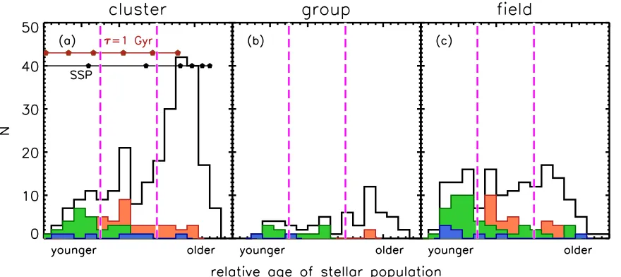
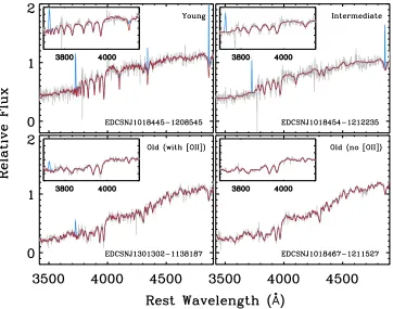
Motivated by these results, we attempt to draw boundaries in this diagram that can separate the galaxies based on a relative measure of the luminosity-weighted stellar age. In Figure2we show a histogram of the log(/)>10.4 galaxies along this sequence, running from the upper left to lower right. The population of older galaxies is clearly identifiable in the clusters and groups as being the dominant population by numbers. By contrast, in the field the relative numbers of galaxies are roughly constant as a function of age. To isolate galaxies by the luminosity-weighted age of their stellar populations, we delineate three regions along this sequence. The slope of these lines is 7.2. We select galaxies whose light is dominated by old stars by drawing a line in this histogram(and a corresponding diagonal line in Figure 1) that separates the peak of old galaxies from the rest. Using the models from Figure1(d), we see that this division(lower diagonal dashed line) selects galaxies that must have few contributions from young or intermediate-age stellar populations, corresponding to roughly six e-foldings of the SFH. In Figure 3 we show representative spectra for our different classes and show one example each from the “older” class of galaxies with and without emission. The absorption spectra of the two “older” classes show spectra dominated by old stars.

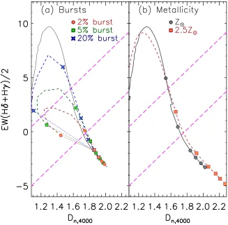
In Figure4 we explore the effects of bursts and metallicity on the location of objects in theDn(4000)–áHdabsHgabsñplane.

In order to meet our Dn(4000)–áHdabsHgabsñcriteria for older

ages, no more than 2% of the stars can have been formed in the past 1 Gyr from a burst superimposed on a 3 Gyr old passively evolving solar metallicity population. We also explore the effect of metallicity, as that will shift the models to larger

metallicity of 2.5Z_e must have experienced their last major epoch of star formation at least 1.5 Gyr before the epoch of observation. In comparison, SSPs with solar metallicity enter the lower right region of the plot 2.5 Gyr after their formation. Galaxies with a superimposed burst on an older population require less time to enter this region (Figure 4, left panel) because their is a substantial contribution to the total light from the preexisting population, which accelerates the evolution in theDn(4000)–áHdabsHgabsñplane. As the galaxies in this region

are not truly old but merely have a lack of young and intermediate-age stellar populations, we designate this the “older”region.

The remaining space is split between the “younger” and “intermediate”regions. The dividing line between “younger” and “intermediate” has been chosen to be approximately between theáHdabsHgabsñand Dn(4000)values for a 6 Gyr old population with a constant SFR model and those for an exponentially declining SFR model with an exponential timescale of 2 Gyr. Changing the exact location or slopes of the dividing lines does not significantly affect our results.

The age interpretation of our stellar index measurements is consistent with the measured strength of[OII]in our galaxies,

as the fraction of [OII]emitters and the characteristic EW([OII])decreases toward older stellar ages. However, there is a population of emission-line galaxies at old ages. They are the main focus of this paper and will be discussed in subsequent sections.

3.2.1. The Colors of Galaxies with Different Spectral Types

A major advantage of our indices is that they are less susceptible to dust than broadband colors, as they each probe a small wavelength baseline. We quantify this in Figure5, where we plot color–magnitude diagrams for galaxies classified by environment, EW([OII]), and relative age of stellar populations

(see Section3.2). We define the red sequence byfitting to the population of cluster galaxies with old spectroscopic ages and no emission. For all three environments these galaxies fall on the same red sequence with equal scatter around this line. For our“intermediate”-age bin we find that many of the galaxies would be classified as red sequence objects even though they have had significant star formation within the past 1 Gyr and often have emission lines. Many of these red “intermediate” -age galaxies have significant obscuration, which drives their Figure 1.Plot of the average of the equivalent width of EW(Hδabs)and EW(Hγabs)vs.Dn(4000)for(a)cluster,(b)group, and(c)field galaxies. All emission and

absorption features have been decomposed as described in the text. Only galaxies with log(/)>10.4 are plotted. The color of the points indicates EW([OII])

red colors(G. Rudnick et al. 2017, in preparation). Some subset may also be recently quenched. It seems therefore clear that our spectroscopic selection, when compared to a simple single

color selection, provides a more robust way to select truly passive galaxies with no young stellar populations.

4. The Environmental Dependence of Galaxies with Old Stars and Weak Emission

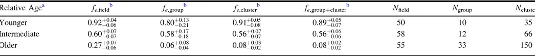
In Figures 1,2, and5, it is apparent that there are galaxies with weak emission lines and old stellar ages. These emission-line galaxies are present in roughly equal numbers in the field and in clusters and are nearly absent in groups. Already from thesefigures you can see that the very different total number of “older”galaxies implies that the fraction of such galaxies with emission must depend greatly on environment. We quantify this result in Figure6, where we plot the fraction of galaxies with [OII] emission as a function of age. Among the three environments, there are no differences in the fractions for galaxies with“younger”or “intermediate”ages. However, for the “older”population of galaxies, there is a difference in the fraction with EW([OII])>5Å, which we callfoe. The value of 5Åis the equivalent width limit above which we can reliably identify and fit the[OII]line.

In thefield the fraction of“older”galaxies with emission is

foe,field=0.27-+0.06

0.07_{, while in clusters and groups f}

oe,clusters=

-+

0.08 0.020.03 and foe,groups=0.06-+0.040.08, respectively. Phrased

dif-ferently, thefield has a 2.7σhigher fraction of old emission-line galaxies when compared to the cluster galaxies and a 2.1σ higher fraction when compared to group galaxies. When combining group and cluster galaxies together, the difference with respect to the field changes to a 2.8σ difference. We provide the fractions of [OII] emitters in Table 3. It is important to remember that our field galaxies are excluded from lying in groups or clusters and therefore indicate a true field sample.

We test for a stellar mass dependence in the emission-line fractions. We divide the sample into two bins of stellar mass split at log(/)=11.0 and find that the results in the two stellar mass bins are consistent with results for the whole sample, although with lower statistical significance. This conclusion does not depend on the exact definition of the stellar mass bins. We have also tested to see whether the stellar mass distributions of the samples in different environments are different. Using a K-S test, the stellar mass distributions for all “older”galaxies in clusters and thefield have a 13% probability of being drawn from the same underlying distribution. Likewise, the “older” emission-line galaxies in clusters and thefield have an 18% probability of being drawn from the same distribution.

A potential concern is that our result may be dominated by a subset of the systems in each environmental bin. In Figure7we address this by showing the emission-line fractions among “older”galaxies for each system independently. Wefind that all of the individual clusters and groups are below the value of the field, implying that our result is true for the whole population of galaxies and is not just dominated by a few specific structures. It is perhaps interesting that the two most massive clusters show a lower fraction of[OII]emitters than lower-mass clusters. This is reminiscent of the results of Poggianti et al.(2006), who used the same cluster sample as in this work to conclude that the fractions of [OII] emitters for galaxies of all ages were lower for more massive clusters. Although their measures of EW([OII]) are systematically different from ours and were conducted on a luminosity-selected sample, it is still interesting that this mass dependence may persist even for galaxies such as ours with extremely weak emission and old stellar populations.

In addition to measuring the fraction of emission, it is also instructive to look at the distribution of EW([OII]). In Figure8 we show the distribution of EW([OII]) in our mass-selected sample of“older”galaxies with EW([OII])>5Å. As there are almost no “older” galaxies in our groups that meet this Figure 2.Histogram of galaxies along the direction of the sequence in Hδabsand Hγabsabsorption line strength(áHdabsHgabsñ)andDn(4000) (see Figure1). Thex-axis

EW([OII])threshold, we can only examine the distribution of clusters and the field. The cluster galaxies are shifted to systematically lower EW([OII])values than the field, and the K-S probability that they are drawn from the same distribution is 3%. The median EW([OII]) of the cluster and field population are slightly different at 6.3 and 8.8Å, respectively, but the 68% limits on the two distributions overlap signifi -cantly. It is therefore difficult to draw any strong conclusions about the distribution of EW([OII]) in the different environ-ments, but we will discuss a possible origin for this shift in Section 5.

4.1. Radial and Velocity Distributions of Different Populations

In order to gain insights as to the infall history of the different populations in Figure 9, we examine the projected phase-space locations of the different galaxy populations. We limit ourselves to clusters, as they are the only systems with enough members for us to reliably determineσand henceR200.

We also remove the cluster Cl 1138.2-1133a, as it is too off-center in our spectroscopic observations to probe out toR200.

This diagram has been used by multiple authors to understand the orbital state of cluster galaxies(e.g., Mahajan et al.2011; Haines et al. 2012; Oman et al. 2013). In those papers the authors used simulations to establish that the regions with small projected radii (Rproj/R200<1.0) and small velocities

(∣Dv∣ s<2) contain most of the virialized galaxies, while moving toward higher velocities or larger radii corresponds to galaxies that either are infalling for the first time or have just finished theirfirst pass through the cluster center(the latter are often called “back-splash”galaxies). In Figure 9 we indicate the corresponding virialized region from Mahajan et al.(2011).

One must exercise caution in tying locations in this diagram directly to a time since infall, as Oman et al. (2013) showed that the distribution of infall times at any given projected position–velocity space is very broad. Nonetheless, galaxies lying within the curve in the left panel of Figure9are strongly preferred to have been in the cluster for greater than 3 Gyr. In Figure 10, we also plot the cumulative distributions of the different populations both in projected radius in units of R200

and in radial velocity in units of the cluster velocity dispersion. With the caveats above in mind, we find that our “older” population preferentially occupies the virialized region of the diagram. In contrast, both the “younger” and “intermediate” galaxies, regardless of the presence of emission lines, and “older”emission-line galaxies are largely absent from regions with lowRproj<R200(Figure10). We test the significance of

the distributions in phase space andfind that the“younger”+ “intermediate” and “older” galaxies have a <2×10−3 K-S probability of having been drawn from the same distribution in projected clustercentric radius. In contrast, the “older” emis-sion-line galaxies are completely consistent with the “ young-er”+“intermediate” galaxies and only marginally so

(PK S‐ »3.1%) with the “older” galaxies. A K-S test on the absolute value of the velocity relative to the cluster velocity dispersion (Figure 10, right panel) shows that all of the populations are consistent at the greater than 17% level with being drawn from the same population. We perform a third test in which we compute the shortest(or perpendicular)distance of each point to the nearest segment of the Mahajan et al.(2011) curve, where this distance is measured in the axis units of Figure9, and assign negative distances to those galaxies inside the curve. This is a measure in phase space of the distance from the virial region and combines velocity and position. A K-S test Figure 3.Typical example spectra for galaxies in each of our three different absorption-line spectral classifications. For the“older”sample, we also show an example of a galaxy with an old stellar spectrum and with[OII]emission. The gray curve represents the data. The red curve represents the modelfit to the spectrum excluding the wavelengths where emission lines are expected. Blue curves show significantly detected emission lines. The inset in each panel is a zoom into the region around the Hδand Hγlines andDn(4000).

of the distributions of this distance shows that the “older” emission-line galaxies and “younger”galaxies are completely consistent while the “older” emission-line galaxies are only marginally consistent with the general “older” population

(PK S‐ »6.7%). As with the pure radial distributions, the “younger” and “older” galaxies have a <2×10−3K-S probability of being drawn from the same distribution.

5. Discussion

As outlined in the previous sections, we have found that galaxies dominated by old stellar populations are more likely to have [OII] emission in field environments than in group or clusters. The first impulse is to attribute this effect to an environmental signature, given the differences with environ-ment. However, in determining the origin and cause of the observed difference in emission we examine a range of possibilities. Our goal is not simply to pick one scenario that is consistent with our observed environmental dependence in the EW([OII]) distribution, but rather to test a large range of possible explanations and see what is required by the data, what is allowed, and what is ruled out. Given the subtle nature of environmental effects, we feel that it is important to carefully examine many alternative possibilities. We proceed using a decision tree that outlines the path to our conclusions. A graphical representation of this tree is given in Figure 11, which identifies the sections that refer to each branch of the

tree. We now address these in turn, starting from the top of the tree.

5.1. Are the Differences in[OII]Fraction Driven by Gas Content or Excitation?

In this subsection we will first address the source of the excitation. We will then discuss whether this excitation source can be different in different environments, and we will close by concluding that differences in gas content must be driving the differences in the[OII]fractions.

5.1.1. Source of the Excitation

Local studies have made significant progress toward under-standing the sources of gas excitation in red galaxies. Many line diagnostics have been used to study the emission mechanisms in red local galaxies (e.g., Sarzi et al. 2006; Yan et al.2006; Stasińska et al.2008; Sarzi et al.2010; Stasińska et al. 2015), but as only ≈50% of our spectra with an [OII]

detection go to long enough wavelengths to measure even Hβ, we cannot use the same line diagnostics as those authors for all our sources. Instead, we use a modified version of the Yan et al.

(2006) diagnostic that was developed by Sánchez-Blázquez et al. (2009). This diagnostic works because star formation under normal extinction conditions is not able to produce EW([OII])/EW(Hβem)>6.7 (e.g., Moustakas et al. 2006;

Sánchez-Blázquez et al.2009). We plot this ratio as a function of EW(Hβem) for our sources in Figure 12. We include 1σ

lower limits on the ratio for galaxies with no detected Hβ. We see that the “older” galaxies are near to or above this line, implying that the excitation is likely not caused by star formation. We also verify that these results are unchanged if we plot the ratio of[OII]to Hβfluxes instead of equivalent widths. We further test the lack of star formation by searching for MIPS 24μm detections in our “older”galaxies with emission lines, using the deep MIPS data on our clusters from Finn et al.

(2010). These data have an infrared luminosity (LIR) 80%

completeness limit of 8.1×1010L_e, corresponding to an SFR limit of ≈8yr−1. We find that only one of the “older” cluster galaxies with[OII]emission(8%)and one in thefield

(7%)have an MIPS 24μm detection, while zero of our“older” emission-line galaxies are detected at 24μm in groups. In contrast, we find that between 43% and 71% of our “intermediate”galaxies with[OII]emission lines are detected with MIPS in the different environments, while 69%–75% of

our “younger” galaxies with [OII] emission are detected, consistent with the “intermediate” and “younger” galaxies having significant ongoing star formation. The EW([OII])

values for“older”galaxies are lower than for the other two age bins. We therefore also test whether this difference in the EW([OII]) values can account for the different fraction of MIPS detections. We find that those galaxies with 5<EW

([OII])/Å<10 in the “intermediate” and “younger” age groups have MIPS detection fractions between 33% and 100% depending on the age and environment bin. This is significantly higher than for“older” galaxies in any environ-ment and indicates that weak [OII] emitters in the “ inter-mediate”and“younger”age groups, regardless of environment, are more likely to have their[OII] emission powered by star formation. Likewise, this implies that the [OII] emission in “older” galaxies is not coming from highly obscured star formation embedded in an older stellar cocoon.

This is consistent with studies of the excitation source in local red galaxies. Yan et al.(2006)found that many of the red Figure 5.Color–mass plot for cluster, group, andfield galaxies divided into bins of relative age as described in the text. The yellow solid lines are identical in each panel and show a robust linearfit to the“older”galaxies in clusters, and the dotted lines are spaced at±0.3 mag. This encompasses nearly all of our“older”objects. There are many objects on the red sequence with significant populations of intermediate-age stars(middle column). These galaxies are biased toward the blue side of the red sequence. This implies that color selection in all environments probes a significant range in ages. The“older”galaxies with emission—the focus of this paper— trace the whole sample of“older”galaxies.

galaxies in the SDSS with weak [OII] emission (similar in strength to our EW([OII])) had line ratios consistent with a LINER-like spectrum(Heckman1980). Sarzi et al.(2006)and Sarzi et al.(2010)used SAURON integralfield spectroscopy of nearby early-type galaxies to demonstrate that much of the ionized emission in early types with a LINER-like spectrum is extended and traces the stellar light. They therefore concluded that the heating source is consistent with post-asymptotic giant branch (pAGB) stars and not an AGN.17 This finding is consistent with work by Annibali et al.(2010), who used long-slit spectroscopy of local early types, with Yan & Blanton

(2012), who used SDSS spectroscopy of 500 passive galaxies observed as part of the Palomar Survey (Ho et al.1995), and with Singh et al.(2013)and Kehrig et al.(2012), who studied the spatially resolved emission-line properties of galaxies in the CALIFA survey(Sánchez et al.2012). Shocks are not a likely excitation source for this emission, as the necessary shock velocities are not consistent with the observed gas kinematics

(Sarzi et al.2010; Yan & Blanton2012).

To further test whether our sources are consistent with a pAGB emission mechanism, we compare the [OIII] strength

from Sarzi et al.(2010)with that predicted for our galaxies. We do this as we only have access to[OIII]for a handful of sources

(but see below) and because Sarzi et al. (2010) do not have access to[OII]. We start with the typical EW([OIII])values of 1–2Å from Sarzi et al. (2010). We then use the LINER line ratios from Heckman (1980), who find that L([OII])/L ([OIII])∼2–4. Given the typical continuum ratios between [OIII] and [OII] in our “older” galaxies of ∼3, this implies EW([OII]) for LINER-like galaxies of 6–24Å, which is consistent with the distribution of EW([OII]) seen in Figure 8. This implies that our emission is consistent with a LINER-like spectrum that is produced by pAGB heating. As an additional check, in Figure13we show that EW([OIII])for our “older” galaxies has values typically consistent with being powered by pAGB stars (EW([OIII])<2Å), with ∼20% of the galaxies having EW([OIII])that implies an AGN contrib-ution. If we instead comparef([OII])tof([OIII]), wefind that 30% of our sources have EW([OIII]) that implies an AGN contribution. The spatial resolution of our spectroscopy is not high enough to address the spatial extent of the emission, and we can therefore only conclude that the emission is likely not related to star formation but comes either from a weak AGN or from the heating of gas by pAGB stars.

That the emission does not come from star formation in our “older”galaxies is also consistent with the observed values of

Dn(4000)andáHdabsHgabsñ, as we show in Figure4that even a

small amount of ongoing star formation is enough to move our galaxies out of the“older”bin. As afinal support that the weak [OII] emission is not coming from star formation, Sánchez-Blázquez et al.(2009)used indices to measure the ages of red sequence galaxies in our same clusters—indeed, for many of the same galaxies—andfind that the luminosity-weighted mean stellar age of their cluster galaxies does not change when excluding those red sequence galaxies with weak emission. This further bolsters our claim that the emission is not coming from small amounts of star formation. It is, of course, possible that galaxies with small amounts of star formation could temporarily leave our “older” bin and be excluded from our analysis, but this does not alter the significant difference in the [OII] fraction among older galaxies seen in different environments.

Jaffé et al. (2014) also analyzed morphologically selected early-type galaxies in EDisCS with extended emission. They concluded that the emission from their sample was powered predominantly by star formation and not by evolved stellar populations. This conclusion was based both on the blue colors of the galaxies and on the fact that they fell predominantly in the“intermediate”and“younger”section defined by this paper in theDn(4000)–áHdabsHgabsñplane. Indeed, only four of their

galaxies would have entered our “older” sample. It is also worth noting that 10 of their 18 early-type galaxies have EW

([OIII])>10Å, and four would not have met our EW([OII])>5Å limit. Therefore, 4/14=30% of their sample has 5Å<EW([OII])<10Å, compared to 74% for our sample. We can therefore say with confidence that our samples are largely disjoint and that they are focused on early types with residual star formation, whereas we are focusing on galaxies with no recent star formation. Nonetheless, their results have implications for gas processes in clusters, which we will address in subsequent sections.

Figure 6.Fraction of galaxies with EW([OII])>5Åas a function of relative stellar population age as defined in Figures1and2. The points have been shifted in thex-direction slightly with respect to one another so that they do not overlap. This plot demonstrates one of the key results of the paper, namely, that old galaxies in the field have a higher fraction of[OII]emission than old galaxies in clusters and groups.

17

There are multiple potential sources of UV ionization and excitation in passive galaxies, including extremely blue horizontal branch stars, and multiple

Table 2

Galaxy Data

ID zspec EW([OII])a EW([OIII])b EW(Hβem) EW(Hδabs) EW(Hγabs) Dn(4000) log(M_* M) Environment

(Å) (Å) (Å) (Å)

EDCSNJ1018471-1210513 0.4716 6.64±1.20 L 1.42±0.33 1.37±0.60 −1.57±0.61 1.68±0.03 10.97 Cluster

EDCSNJ1018464-1211205 0.4717 <0.77 L L −0.05±1.03 −4.93±1.08 1.93±0.07 10.61 Cluster

EDCSNJ1018467-1211527 0.4716 <0.51 L L −1.13±0.37 −5.55±0.37 1.96±0.03 11.63 Cluster

EDCSNJ1018454-1212235 0.4789 6.48±0.66 1.34±0.36 3.59±0.25 2.82±0.43 1.29±0.38 1.31±0.02 10.94 Cluster

EDCSNJ1018438-1212352 0.4732 <1.10 L L 2.60±0.90 −2.50±0.90 1.67±0.05 10.52 Cluster

Notes.All galaxies with EW([OII])<5Åhave been replaced by their 1σupper limits. All galaxies with EW(Hβem)measurements that are less than 2σare replaced by the 1σupper limits. No entry for a given line

indicates that the specified feature did not fall in the wavelength range of the spectrum.

a

[OII]λ3727.

b

[OIII]λλ4959, 5007.

(This table is available in its entirety in machine-readable form.)

12

The

Astrophysical

Journal,

850:181

(

22pp

)

,

2017

December

1

Rudnick

et

5.1.2. Could the pAGB Properties Be Different in Different Environments?

If we assume that the emission in our “older” galaxies is indeed powered by pAGB stars, the next question is whether the pAGB properties could be different in different environ-ments. One possibility to explain the difference in pAGB properties would be if the stellar IMF were different in the various environments, as different abundances of low-mass stars would influence the number of UV-emitting evolved stars

(pAGB or horizontal branch[HB]stars). Indeed, Zaritsky et al.

(2014, 2015)have shown that the total mass-to-light ratio of

early-type galaxies drawn from the SAURON and ATLAS3D samples correlates strongly with UV color, implying that the low-mass IMF slope partially controls the UV emission properties in early-type galaxies. They propose that the UV slope could actually test for IMF differences. Unfortunately, we do not have rest-frame UV photometry for our galaxies and can therefore not directly test whether the IMF is different for galaxies in different environments. However, there is no reason to assume that the galaxies in groups and clusters in our sample have different IMFs. The mean velocity dispersions for cluster andfield early-type galaxies in EDisCS above our stellar mass limit are within 0.05dex of each other(Saglia et al.2010). This implies at most a ∼0.03 dex systematic difference in the total mass-to-light ratios(Zaritsky et al.2015). We therefore have no evidence that differences in the spectrum caused by IMF differences can explain the observed differences in the EW([OII])distributions.

The only properties of the stellar population that could conceivably be different in different environments are the SFH and metallicity. Regarding the latter, the mass range of our sample(log(/)>10.4)makes it unlikely that there are substantial metallicity variations. Regarding possible SFH differences, the number of pAGB stars in a stellar population, and hence their contribution to the UV radiationfield, changes with stellar age. Binette et al. (1994) have one of the most recent determinations of this contribution andfind that the UV continuum output of pAGB stars changes by∼15% for stellar populations between 1 and 8 Gyr, spanning the full possible range of age differences in our sample as governed by our

Dn(4000)–áHdabsHgabsñselection and a formation redshift of 6.

However, these changes occur in an opposite sense shortward and longward of Lyα, such that they mostly cancel out in terms of the total UV energy input(Binette et al.1994).

Despite the small expected difference in the pAGBflux, we nonetheless attempt to further constrain the potential age differences between different environments. By virtue of their selection in Dn(4000) and áHdabsHgabsñ strength, the “older”

galaxies in our different environmental bins are already

constrained to have roughly similar ages. They also have the same peak in their distributions in the Dn(4000)–áHdabsHgabsñ

plane(see Figure2), ruling out any large differences within this larger age bin. Nonetheless, there may be small age differences between passive galaxies in different environments. Drawing from the literature, van Dokkum & van der Marel (2007) performed a fundamental plane comparison of visually classified massive E/S0 galaxies in the field and in rich clusters atz<1 and found that the luminosity-weighted ages between these two populations differed by only 4%. This small age difference makes it unlikely that there could be large differences in the pAGB population driving the changes in the [OII]fraction.

On the other hand, Saglia et al. (2010) measured the fundamental plane for the EDisCS clusters used in this analysis and found that the size at a fixed dynamical or stellar mass increases with decreasing redshift. Taking this into account and performing a consistent comparison betweenfield and cluster galaxies, they found that thefield galaxies were approximately 1–2 Gyr younger than the cluster galaxies at a fixed stellar mass. The origin of the difference between Saglia et al.(2010) and van Dokkum & van der Marel(2007)is not clear. Perhaps it stems from the latter using much more massive clusters than the former, as there is some tentative evidence for different speeds of the buildup of the red sequence in low- and high-mass clusters (De Lucia et al. 2007; Gilbank et al. 2008; Rudnick et al. 2009). Additionally, van Dokkum & van der Marel(2007)assumed homology, i.e., no size evolution in the early-type population at afixed surface brightness and velocity dispersion, whereas Saglia et al. (2010) allowed for size evolution. This may result in different estimates for the stellar population ages derived using the fundamental plane evolution. We adopt the results from Saglia et al.(2010)as an indication of the maximum age difference between cluster and field galaxies and explore the consequences below. Unfortunately, the quality of the EDisCS data also precludes a precise estimate of the stellar population age differences between old galaxies with and without weak emission lines(Sánchez-Blázquez et al. 2009).

It is not possible to easily convert this age difference into a difference in expected[OII]fractions, as the modeling of the UV contribution of pAGB stars is still very uncertain. Brown et al.(2008)find far fewer pAGB stars in M32 than expected by theoretical models, and similar in abundance to more recent observational studies of M31 by Rosenfield et al.(2012). Other authors have pointed out that the pAGB contributions to the Lyman continuum of galaxies is uncertain at the factor of∼2 level (Stasińska et al. 2008; Cid Fernandes et al. 2011; Papaderos et al.2013). However, we can investigate whether Table 3

Fractions of Emission-line Galaxies as a Function of Stellar Age and Environment

Relative Agea fe,field

b

fe,group

b

fe,cluster

b

fe,group+cluster

b

Nfield Ngroup Ncluster

Younger 0.92-+0.060.04 0.80-+0.210.13 0.91+-0.080.05 0.89-+0.070.05 50 10 35

Intermediate 0.60-+0.070.07 0.58-+0.180.17 0.56+-0.070.07 0.56-+0.060.06 58 12 66

Older 0.27-+0.060.07 0.06-+0.040.08 0.08-+0.020.03 0.08-+0.020.02 55 33 150

Notes.All errors on the fractions are computed using binomial errors. Galaxies are limited in stellar mass to log(/)>10.4. The numbers in the rightmost columns correspond to the total number of galaxies in each age–environment combination that pass all of our selection criteria.

a

The relative ages corresponding to the age divisions in theDn(4000)–áHdabsHgabsñplane as shown in Figures1and2. b

this age difference can result in a significant difference in the number of young stars, under the assumption that they may contribute somewhat to the[OII]excitation mechanism if they exist in small proportions. According to Figure 1(d), galaxies

need at least six e-foldings of their SFH to enter the “older” region of the Dn(4000)–áHdabsHgabsñ plane. For a τ=1 Gyr

exponential SFH(red curve in Figure 1(d)), the mass fraction of stars younger than 1 Gyr decreases from 0.5% for a 6 Gyr old population to 0.2% for a 7 Gyr old population. While the fraction of these young stars for a simple tau model is very small, it is systematically different forfield and cluster galaxies. Unfortunately, it is quite complicated to convert this stellar population difference into a difference in the EW([OII])

distribution, especially as we do not know the relative spatial distribution of gas and young stars in our galaxies. This renders us unable to rule out modest age differences contributing somewhat to the difference betweenfield and cluster galaxies. However, because the difference in EW([OII])distributions is also present between groups and the field, it implies that systematic age differences must exist between those two environments if that were to explain our result. Unfortunately, no comparisons of the fundamental plane evolution in groups and the field have been undertaken, making it impossible to determine whether age differences could be explaining the difference in[OII]fractions in those environments. That said, as our groups may not exist in large-scale overdensities, it is not even clear whether we would expect them to have collapsed at an earlier time than ourfield galaxies.

In summary, there may be small age differences for passive galaxies in different environments, but there is no way to directly test the effect of these age differences on the [OII]

fractions. Measuring the [OII] fractions of galaxies in halos with a wider range in mass and large-scale overdensity may help to solve this problem. Additionally tracing the spatial distribution of the small young stellar populations and the gas may enable the use of models to determine whether the[OII]

fraction difference can be caused by age differences. Setting Figure 7.Fraction of“older”galaxies with[OII]emission for all of our groups

and clusters and for thefield. The gray squares are for the individual systems with groups and clusters being divided at 400 km s−1_{. The large yellow}

diamond and large red star are the values for all the galaxies in the group and cluster samples, respectively. The horizontal purple lines indicates the value for thefield and its 68% confidence interval.

Figure 8. Cumulative distributions of EW([OII]) for galaxies with EW([OII])>5Åthat are classified as “older” based on Dn(4000)and the

d g

áHabsHabsñstrength. The cluster+group distribution is shifted toward lower

EW([OII])values, with only a 3% K-S probability of being drawn from the same distribution as thefield galaxies.

Figure 9. Projected phase-space positions of different cluster galaxy populations. The solid curve is from Mahajan et al.(2011)and contains most of the virialized galaxies in their simulations. The purplefilled circles refer to those galaxies in the“younger”and“intermediate”age categories.

those uncertainties aside, we conclude that there are no required mechanisms for a difference in excitation source being responsible for the difference in EW([OII])distributions.

5.2. The Environmental Dependence Is Not Driven by the Morphology–Density Relation

It is well known that the early-type fraction is higher in dense environments than in the field (e.g., Dressler 1980; Postman et al.2005). Therefore, it is important to check that the differences infoeare not merely reflecting the environmentally dependent early-type fraction. We test this using theHST-based visual morphologies available for 11 clusters andfive groups in our sample.

In Figure 14 we show the morphological distribution of “older” galaxies in each environment. A total of 76% of our “older”galaxies are E/S0, and the remaining 24% are mostly Sa with a few Sb galaxies. All but three of our emission-line “older”galaxies are early-type galaxies. The fraction of“older” galaxies that are early types is statistically indistinguishable in the different environments. Also, the fraction of the “older” emission-line galaxies that are early types is ∼80% and is statistically indistinguishable in the different environments. However, when restricting ourselves to early-type galaxies, the difference in the fraction of emission-line galaxies is as significant as for the whole spectroscopic sample.

We therefore conclude that changes in the morphological fraction among our environments are not driving the difference we see in the emission-line fraction.

5.3. The Origin of Differences in Gas Content

As outlined in the previous sections, the difference in the EW([OII]) distributions is due neither to differences in the radiation field nor to differences in the morphological distribution of galaxies in different environments. The remain-ing possibility is that the difference in the EW([OII])

distribution is caused by differences in the gas content. In all galaxies gas is resupplied to the interstellar medium(ISM)via mass loss from stars. For a Chabrier IMF, the total mass returned to the ISM from a simple stellar population reaches 50% at an age of 6 Gyr (Bruzual & Charlot 2003), which corresponds to the time difference between the lowest-redshift end of our sample (z=0.4) and z=1.7.18 In thefirst 1 and 2 Gyr, 80% and 90% of this gas is returned to the ISM, respectively. Therefore, the total gas content changes only by 10% in the time between 2 and 6 Gyr, representing the largest possible difference in gas contents. However, the age difference between the cluster andfield galaxies in our sample is likely significantly less than this(see Section5.1.2), and the difference in gas contents should therefore be correspondingly smaller. It is therefore unlikely that differences in the amount of gas from mass loss resulting from age differences can account for the difference in the observed[OII]fractions.

In this subsection we therefore consider additional external origins for the gas difference and discuss whether the differences represent an excess of gas in field galaxies or an active removal of gas in cluster and group galaxies.

5.3.1. Excess of Gas in Field Galaxies

A possible explanation for the difference in emission-line fractions in old galaxies in different environments is that gas accretion onto satellite galaxies in groups and clusters is no longer efficient. In this picture, the “older” emission-line galaxies that we see in groups and clusters are also likely present in the field and have their gas supply dominated by mass loss from existing stellar populations heated by evolved stellar populations. Given that 90% of the gas is returned in the first gigayear, there should be ample gas to supply this emission. The additional galaxies with emission in the field Figure 10.Left: cumulative histogram ofRproj/R200for the different galaxy populations. All galaxies with emission are systematically biased to large clustercentric

radii. Right: cumulative histogram of∣Dv∣ sfor the same galaxy populations. All of the populations are statistically consistent with being drawn from the same underlying distribution.

18_{Byz=1.7 many red sequence galaxies were already in place(Papovich}

would then come from a population of galaxies that are undergoing accretion of gas directly onto those galaxies, in either a hot or cold mode of accretion. Galaxies in thefield with our stellar mass are likely to be central galaxies of their halos

and so would be the repository of this gas, although it is presumably kept from forming stars by some sort of feedback. Most of our galaxies in groups and clusters, however, are satellites, and the gas that would normally have been deposited Figure 11.Decision tree used in our discussion, outlining all of the major decisions made in coming to our conclusions. The tree starts at the top middle of the box, and the box representing our conclusion is at the lower right. Red boxes represent decision branches, black arrows and accompanying text outline possibilities for each decision, yellow boxes represent that a given choice is not matched by observations, and blue box parallelograms provide information that goes with each choice. Bold and underlined text represents the section of the text that refers to each portion of the tree.