Image and Collateral Text in Support of Auto-annotation and Sentiment
Analysis
Pamela Zontone and Giulia Boato University of Trento
Trento, Italy.
{zontone|boato}@disi.unitn.it
Jonathon Hare and Paul Lewis University of Southampton Southampton, United Kingdom {jsh2|phl}@ecs.soton.ac.uk
Stefan Siersdorfer and Enrico Minack L3S Research Centre
Hannover, Germany
{siersdorfer|minack}@l3s.de
Abstract
We present a brief overview of the way in which image analysis, coupled with associated collateral text, is being used for auto-annotation and sentiment analy-sis. In particular, we describe our ap-proach to auto-annotation using the graph-theoretic dominant set clustering algo-rithm and the annotation of images with sentiment scores from SentiWordNet. Pre-liminary results are given for both, and our planned work aims to explore synergies between the two approaches.
1 Automatic annotation of images using graph-theoretic clustering
Recently, graph-theoretic approaches have be-come popular in the computer vision field. There exist different graph-theoretic clustering algo-rithms such as minimum cut, spectral clustering, dominant set clustering. Among all these algo-rithms, the Dominant Set Clustering (DSC) is a promising graph-theoretic approach based on the notion of a dominant set that has been proposed for different applications, such as image segmen-tation (Pavan and Pelillo, 2003), video summariza-tion (Besiris et al., 2009), etc. Here we describe the application of DSC to image annotation.
1.1 Dominant Set Clustering
The definition of Dominant Set (DS) was intro-duced in (Pavan and Pelillo, 2003). Let us con-sider a set of data samples that have to be clus-tered. These samples can be represented as an undirected edge-weighted (similarity) graph with no self-loopsG= (V, E, w), whereV = 1, . . . , n
is the vertex set, E ⊆ V ×V is the edge set, and w : E → R∗+ is the (positive) weight func-tion. Vertices in G represent the data points,
whereas edges represent neighborhood relation-ships, and finally edge-weights reflect similarity between pairs of linked vertices. Ann×n sym-metric matrix A = (aij), called affinity (or
simi-larity) matrix, can be used to represent the graph
G, whereaij =w(i, j)if(i, j) ∈E, andaij = 0
ifi=j. To define formally a Dominant Set, other parameters have to be introduced. LetSbe a non-empty subset of vertices, withS ⊆V, andi∈S. The (average) weighted degree ofirelative toSis defined as:
awdegS(i) = 1
|S|
X
j∈S aij
where |S|denotes the number of elements in S. It can be observed that awdeg{i}(i) = 0for any
i ∈ V. If j /∈ S we can define the parameter
φS(i, j) = aij −awdegS(i) that is the similarity
between nodesjandiwith respect to the average similarity between nodeiand its neighbors inS. It can be noted thatφ{i}(i, j) =aij, for alli, j∈V
withi 6=j. Now, ifi ∈S, the weightwS(i)ofi
relative toS is:
wS(i) =
n 1 if|S|= 1
P
j∈S\{j}φS\{i}(j, i)wS\{i}(j) otherwise.
This is a recursive equation where to calculate
wS(i)the weights of the setS\{i}are needed. We
can deduce thatwS(i)is a measure of the overall
similarity between the nodeiand the other nodes inS\{i}, considering the overall similarity among the nodes inS\{i}. So, the total weight ofS can be defined as:
W(S) =X
i∈S wS(i).
A non-empty subset of verticesS ⊆ V such that
W(T) > 0for any non-empty T ⊆ S is defined as a dominant set if the following two conditions
are satisfied: 1.∀i∈S,wS(i)>0; and 2.∀i6∈S, wS∪{i}(i)< 0. These conditions characterize the
internal homogeneity of the cluster and the exter-nal inhomogeneity ofS. As a consequence of this definition, a dominant set cluster can be derived from a graph by means of a quadratic program (Pa-van and Pelillo, 2003). Letxbe ann-dimensional vector, where n is the number of vertices of the graph and its components indicate the presence of nodes in the cluster. LetAbe the affinity matrix of the graph. Let us consider the following standard quadratic program:
maxf(x) =xTAx
s.t. x∈∆ (1)
where∆ = {x≥0andeTx= 1}is the standard simplex ofRn. If a pointx∗ ∈ ∆is a local max-imum of f, and σ(x∗) = {i ∈ V : x∗i > 0} is
the support ofx∗, it can be shown that the support
σ(x∗)is a dominant set for the graph. So, a dom-inant set can be derived by solving the equation (1). The following iterative equation can be used to solve (1):
xi(t+ 1) =xi(t)
(Ax(t))i
x(t)TAx(t)
wheretdenotes the number of iterations. To sum-marize the algorithm, a dominant set is found and removed from the graph. A second dominant clus-ter is extracted from the remaining part of the graph, and so on. This procedure finishes when all the elements in the graph have been assigned to a cluster.
1.2 Image annotation using DSC
Here we present an approach to automatically an-notate images using the DSC algorithm. In the initialization phase (training) the image database is split into L smaller subsets, corresponding to the different image categories or visual concepts that characterize the images in the database. In this process only tags are exploited: an image is included in all subsets corresponding to its tags. Given a subset l, the corresponding affinity ma-trix Al is calculated and used by the DSC
algo-rithm. Following (Wang et al., 2008), the ele-ments of the affinity matrix Al = (aij) are
de-fined asaij =e−w(i,j)/r
2
wherew(i, j)represents the similarity function between imagesiandj in the considered subset l, and r > 0 is the scaling factor used as an adjustment function that allows
the control of clustering sensitivity. We use the MPEG.7 descriptors (Sikora, 2001) as features for computing the similarity between images. Follow-ing the DSC approach, we can construct all clus-ters of subsetlwith similar images, and associate them with the tag of subsetl.
In the test phase, a new image is annotated asso-ciating to it the tag of the cluster that best matches the image. To do this, we use a decision algo-rithm based on the computation of the MSE (Mean Square Error), where for each cluster we derive a feature vector that represents all the images in that cluster (e.g., the average of all the feature vectors). The tag of the cluster with smaller MSE is used for the annotation.
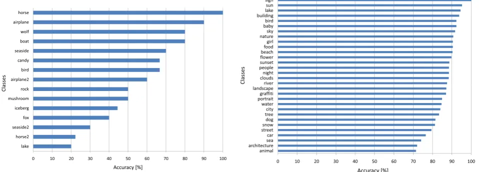
For our experiments, we consider a subset of the Corel database, that consists of 4287 images in 49 categories (L = 49). The 10%of images in each category have been randomly selected from the database and used only for testing. In Fig-ure 1 we report the annotation accuracy results ob-tained on 15 different classes with optimal param-eter r = 0.2. For some classes the accuracy is very high, whereas for others the accuracy is very low (under 30%). The total annotation accuracy considering all the 49 classes is roughly 69%.
In a second set of experiments we consider a set of 6531 images from the MIR Flickr database (Huiskes and Lew, 2008), where each image is tagged with at least one of the chosen 30 visual concepts (L = 30). Images are characterized by multiple tags associated to them, thus an image is included in all the corresponding subsets. For test-ing we use 875 images. To evaluate the annotation accuracy we compare the automatically associated tag with the user defined tags of that image. In Fig-ure 1 we report the annotation accuracy obtained for the 30 different categories, with the optimal pa-rameterr = 0.2. The total annotation accuracy is about 87%.
Further simulations are in progress to evaluate the accuracy of multiple tags that can be associ-ated to the test set in the MIR Flickr database. In-deed, our idea is to annotate the images consider-ing the other common tags of the images belong-ing to each cluster.
2 Annotating Sentiment
Figure 1: Annotation accuracy for 15 classes of the Corel database (left) and for 30 classes of the MIR Flickr database (right).
our work is concerned with opinion analysis in multimedia information and the automatic identi-fication of sentiment. The study of image indexing and retrieval in the library and information science fields has long recognized the importance of sen-timent in image retrieval (J¨orgensen, 2003; Neal, 2006). It is only recently however, that researchers interested in automated image analysis and re-trieval have become interested in the sentiment as-sociated with images (Wang and He, 2008).
To date, investigations that have looked at the association between sentiment and image con-tent have been limited to small datasets (typically much less than 1000) and rather specific, spe-cially designed image features. Recently, we have started to explore how sentiment is related to im-age content using much more generic visual-term based features and much larger datasets collected with the aid of lexical resources such as Senti-WordNet.
2.1 SentiWordNet and Image Databases
SentiWordNet (Esuli and Sebastiani, 2006) is a lexical resource built on top of WordNet. Word-Net (Fellbaum, 1998) is a thesaurus containing textual descriptions of terms and relationships be-tween terms (examples are hypernyms: “car” is a subconcept of “vehicle” or synonyms: “car” de-scribes the same concept as “automobile”). Word-Net distinguishes between different part-of-speech types (verb, noun, adjective, etc.). A synset in WordNet comprises all terms referring to the same concept (e.g.,{car, automobile}). In SentiWord-Net a triple of three senti-values (pos, neg, obj)
(corresponding to positive, negative, or rather neu-tral sentiment flavor of a word respectively) are assigned to each WordNet synset (and, thus, to each term in the synset). The senti-values are in the range of[0,1]and sum up to 1 for each triple. For instance(pos, neg, obj) = (0.875,0.0,0.125) for the term “good” or (0.25,0.375,0.375) for the term “ill”. Senti-values were partly created by human assessors and partly automatically as-signed using an ensemble of different classifiers (see (Esuli, 2008) for an evaluation of these meth-ods).
Popular social websites, such as Flickr, con-tain massive amounts of visual information in the form of photographs. Many of these photographs have been collectively tagged and annotated by members of the respective community. Recently in the image analysis community it has become popular to use Flickr as a resource for building datasets to experiment with. We have been explor-ing how we can crawl Flickr for images that have a strong (positive or negative) sentiment associ-ated with them. Our initial explorations have been based around crawling Flickr for images tagged with words that have very high positive or negative sentiment according to their SentiWordNet classi-fication.
con-positive
[image:4.595.85.518.61.115.2]negative
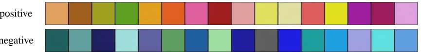
Figure 2: Top 16 most discriminative colours (from left to right) for positive and negative sentiment classes.
tains positive sentiment terms, and a negative (-1) sentiment value if it only contains negative senti-ment terms. We discarded images with neither a positive nor negative score. Currently we are also exploring more powerful ways to assign sentiment values to images.
2.2 Combining Senti-values and Visual Terms
In the future we intend to exploit the use of tech-niques such as the one described in Section 1.2 in order to develop systems that are able to pre-dict sentiment from image features. However, as a preliminary study, we have performed some small-scale experiments on a collection of 10000 images crawled from Flickr in order to try and see whether a primitive visual-bag-of-terms (Sivic and Zisser-man, 2003; Hare and Lewis, 2005) can be asso-ciated with positive and negative sentiment values using a linear Support Vector Machine and Sup-port Vector Regression. The visual-term bag-of-words for the study was based upon a quantisation of each pixel in the images into a set of 64 dis-crete colours (i.e., each pixel corresponds to one of 64 possible visual terms). Our initial results look promising and indicate a considerable cor-relation between the visual bag-of-words and the sentiment scores.
Discriminative Analysis of Visual Features. In our small-scale study we have also performed some analysis in order to investigate which visual-term features are most predictive of the positive and negative sentiment classes. For this analysis we have used the Mutual Information (MI) mea-sure (Manning and Schuetze, 1999; Yang and Ped-ersen, 1997) from information theory which can be interpreted as a measure of how much the joint distribution of features (colour-based visual-terms in our case) deviate from a hypothetical distribu-tion in which features and categories (“positive” and “negative” sentiment) are independent of each other.
Figure 2 illustrates the 16 most discriminative
colours for the positive and negative classes. The dominant visual-term features for positive senti-ment are dominated by earthy colours and skin tones. Conversely, the features for negative sen-timent are dominated by blue and green tones. Interestingly, this association can be explained through intuition because it mirrors human per-ception of warm (positive) and cold (negative) colours.
Currently we are working on expanding our preliminary experiments to a much larger image dataset of over half a million images and incor-porating more powerful visual-term based image features. In addition to seeking improved ways of determining image sentiment for the training set we are planning to combine the dominant set clus-tering approach to annotation presented in Sec-tion 1.2 with the sentiment annotaSec-tion task of this section and compare the combined approach with other state of the art approaches as a step towards achieving robust image sentiment annotation.
3 Conclusions
The use of dominant set clustering as a basis for auto-annotation has shown promise on image col-lections from both Corel and from Flickr. We have also shown how that visual-term feature repretations show some promise as indicators of sen-timent in images. In future work we plan to com-bine these approaches to provide better support for opinion analysis of multimedia web documents.
Acknowledgments
References
D. Besiris, A. Makedonas, G. Economou, and S. Fo-topoulos. 2009. Combining graph connectivity and dominant set clustering for video summarization.
Multimedia Tools and Applications, 44 (2):161–186.
A. Esuli and F. Sebastiani. 2006. Sentiwordnet: A publicly available lexical resource for opinion min-ing. LREC, 6.
Andrea Esuli. 2008. Automatic Generation of
Lexi-cal Resources for Opinion Mining: Models, Algo-rithms and Applications. PhD in Information
Engi-neering, PhD School “Leonardo da Vinci”, Univer-sity of Pisa.
C. Fellbaum. 1998. WordNet: An Electronic Lexical
Database. MIT Press.
Jonathon S. Hare and Paul H. Lewis. 2005. On image retrieval using salient regions with vector-spaces and latent semantics. In Wee Kheng Leow, Michael S. Lew, Tat-Seng Chua, Wei-Ying Ma, Lekha Chaisorn, and Erwin M. Bakker, editors,
CIVR, volume 3568 of LNCS, pages 540–549,
Sin-gapore. Springer.
Mark J. Huiskes and Michael S. Lew. 2008. The MIR Flickr Retrieval Evaluation. In MIR ’08:
Proceed-ings of the 2008 ACM International Conference on Multimedia Information Retrieval, New York, NY,
USA. ACM.
Corinne J¨orgensen. 2003. Image Retrieval: Theory
and Research. Scarecrow Press, Lanham, MD.
C. Manning and H. Schuetze. 1999. Foundations of Statistical Natural Language Processing. MIT
Press.
Diane Neal. 2006. News Photography Image Retrieval
Practices: Locus of Control in Two Contexts. Ph.D.
thesis, University of North Texas, Denton, TX.
M. Pavan and M. Pelillo. 2003. A new graph-theoretic approach to clustering and segmentation.
IEEE Conf. Computer Vision and Pattern Recogni-tion, 1:145–152.
Thomas Sikora. 2001. The mpeg-7 visual standard for content description - an overview. IEEE Trans.
Cir-cuits and Systems for Video Technology, 11 (6):262–
282.
J Sivic and A Zisserman. 2003. Video google: A text retrieval approach to object matching in videos. In
ICCV, pages 1470–1477, October.
Weining Wang and Qianhua He. 2008. A survey on emotional semantic image retrieval. In ICIP, pages 117–120, San Diego, USA. IEEE.
M. Wang, Z. Ye, Y. Wang, and S. Wang. 2008. Domi-nant sets clustering for image retrieval. Signal
Pro-cessing, 88 (11):2843–2849.