Fractional Integration of the Price Dividend Ratio in a Present Value Model

Munich Personal RePEc Archive

Fractional Integration of the

Price-Dividend Ratio in a Present-Value

Model.

Golinski, Adam and Madeira, Joao and Rambaccussing,

Dooruj

University of York, University of York, University of Dundee

13 September 2014

Online at

https://mpra.ub.uni-muenchen.de/58554/

Fractional Integration of the

Price-Dividend Ratio in a Present-Value

Model of Stock Prices

Adam Goli´nski, João Madeira and Dooruj Rambaccussing

12 September 2014

Abstract

We re-examine the dynamics of returns and dividend growth within the present-value framework of stock prices. We …nd that the …nite sample order of integration of returns is approximately equal to the order of integration of the …rst-di¤erenced price-dividend ratio. As such, the traditional return fore-casting regressions based on the price-dividend ratio are invalid. Moreover, the nonstationary long memory behaviour of the price-dividend ratio induces antipersistence in returns. This suggests that expected returns should be mod-elled as an ARF I M A_{process and we show this improves the forecast ability} of the present-value model in-sample and out-of-sample.

JEL Classi…cation: G12, C32, C58

Keywords:price-dividend ratio, persistence, fractional integration, return predictability, present-value model.

1

Introduction

The price-dividend ratio has been shown to have strong forecasting power of future returns at long horizons (see Fama and French (1988a) and Cochrane (1999)). The prediction properties of the price-dividend ratio have a strong theoretical foundation grounded in the present-value (PV) identity, popularized in the log linear form by Campbell and Shiller (1988). As shown in Cochrane (2005), price-dividend ratios "can only move at all if they forecast future returns, if they forecast future dividend growth, or if there is a bubble – if the price-dividend ratio is nonstationary and is expected to grow explosively". Cochrane (2008a) argues that the lack of predictabil-ity of dividend growth reinforces the evidence for forecastabilpredictabil-ity of stock returns. However, many research studies have pointed out that return predictability has been overstated due to the highly persistent price-dividend ratio (e.g. Stambaugh (1986), Stambaugh (1999), Mankiw and Shapiro (1986), Hodrick (1992) and Goyal and Welch (2003)).

relation between returns, dividend growth and price-dividend ratio implies that the order of integration of returns is (in …nite sample) approximately equal to the order of integration of the …rst di¤erenced price-dividend ratio. We …nd the time series of returns to be integrated of order -0.2, con…rming this conjecture.2

The fact that the variables in simple linear regression have di¤erent orders of integration invalidates statistical inference (see Maynard and Phillips (2001)). The negative fractional order of integration in returns and dividend growth in the data must be taken into account when estimating the PV model of stock prices. This motivates specifying the expected return and expected dividend growth series in a PV model as autoregressive fractionally integrated moving average (ARF IM A) processes. We derive the unobserved series for expected returns and expected divi-dend growth through a structural state-space approach. The state-space (or latent-variables) representation has shown to be a ‘useful structure for understanding and interpreting forecasting relations’ as stated by Cochrane (2008b). Recent important examples of this include Van Binsbergen and Koijen (2010) and Rytchkov (2012), who found the state-space methodology to be able to increase the return forecastR2

over price-dividend ratio regressions. As in these papers, we specify expected returns and expected dividend growth as latent variables de…ned within a PV model of the aggregate stock market to which we subsequently apply the Kalman …lter and obtain parameter estimates through maximum likelihood.

The fractional integration parameter in expected returns is found to be statisti-cally signi…cant and negative. Using model selection criteria we …nd theARF IM A(1; ;0)

re-turns follow an autoregressive process of order one results inR2 _{values ranging from} 13to 14 percent for returns and about32percent for dividend growth rates in the 1926-2011 sample. The use of an autoregressive fractionally integrated process in ex-pected returns results inR2 values for returns of about20percent and a range of36

to38percent for dividend growth rates in the 1926-2011 sample. Several prediction exercises on the last40years of data (1971 2011) con…rm the relevance of using a model which accounts for fractional integration in improving the forecast ability of the PV model both in-sample and out-of-sample. Assuming a …rst order autoregres-sive process of expected returns results inR2 _{values of about3 percent for returns}

and a range of11to15percent for dividend growth rates in-sample and negativeR2

for returns and about7 to 12 percent for dividend growth rates out-of-sample. On the other hand, the use of anARF IM A process in expected returns results inR2

values for returns of about9percent and about13to17percent for dividend growth rates in-sample, and out-of-sampleR2_{values of about1to4percent for returns and} 9to13percent for dividend growth.

Using Mincer-Zarnowitz style regressions (Mincer and Zarnowitz (1969)) we check that our model produces latent counterparts that jointly match the time series proper-ties of returns and dividends very well. The expected returns and expected dividend growth series forecast observed series better than the AR(1) model by Van Bins-bergen and Koijen (2010) both in-sample and out-of-sample. Our …ltered series of expected returns and expected dividend growth are clearly countercyclical, which is in line with many other studies (e.g. Chen, Roll and Ross (1986), Fama and French (1989), Fama (1990), Barro (1990)).3

results support to the view that fractional integration processes are relevant in asset pricing.

The remainder of the paper is organized as follows. Section 2 explores the po-tential imbalance in the return forecasting regression due to the high persistence in the price-dividend ratio. In section 3 we set out the PV model withARF IM A dy-namics. In section 4.1 we describe the data. Section 4.2 describes the estimation methodology and results while in section 4.3 we present a series of diagnostics of the model. Section 4.4 presents the out-of-sample performance of particular models. We examine the business cycle ‡uctuations of the model implied expected returns and dividend growth in Section 4.5. Section 5 concludes.

2

The implications of persistence in the price-dividend ratio

We start by de…ning the aggregate stock market’s total log return (rt+1) and log

dividend growth rate ( dt+1) as:

rt+1 log

Pt+1+Dt+1

Pt ; (1)

dt+1 log

Dt+1

Dt : (2)

The price-dividend ratio (P Dt) is:

P Dt Pt Dt:

Usingpdt log(P Dt)and (2) one can then re-write the log-linearized return (1) as:

withpd=E(pdt), = log(1 + exp(pd)) pd; and = _1+exp(exp(pd_pd)₎ (see Campbell and Shiller (1988)).

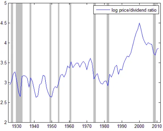
We now proceed to the analysis of the data (see section 4.1 for details). Figure 1 shows the time series for the log of the price-dividend ratio. The price-dividend ratio is lower preceding economic booms and high values preceding recessions, suggesting it could be relevant for forecasting returns. One can also observe that it is a very persistent variable. In Table 1 we report the results of the following regression:

pdt+1= + pdt+ut+1: (4)

The estimated coe¢cient on the lagged price-dividend value is very close to one (0.9417). Table 1 also reports the results of the Augmented Dickey-Fuller unit root test (Dickey and Fuller (1979)). The t statistic ( 1:52) is much smaller than the

5%critical value ( 2:9), which means that we cannot reject the null of a unit root in the series.5 _{Thus, in principle the nonstationarity of the price-dividend ratio}

invalidates a return forecasting regression (see Granger and Newbold (1974)) of the type considered by Fama and French (1988a):

rt+1= + pdt+ut+1: (5)

growth series obtained using three di¤erent semi-parametric estimators, proposed by Geweke and Porter-Hudak (1983), Robinson (1995) and Shimotsu (2010). The Shimotsu estimator, as opposed to the other two, has been designed to deal with a nonstationary time series. As can be seen, the estimates of the fractional parameter ( ) revolve around 0.8, meaning that the series is a nonstationary but mean-reverting process. On the other hand, the time series of returns and dividend growth seem to exhibit antipersistence (i.e. are integrated of order smaller than zero). Inference and forecasting based on estimates of (5) is therefore invalid (as shown by Maynard and Phillips (2001)) due to the di¤erent order of integration of the variables included in it.

At this point, we should consider as well the balance in the order of integration in the log-linearized return equation, (3). A closer inspection of (3) reveals that, due to the discount parameter ( ) being very close to unity, the return series is (almost) over-di¤erenced. Indeed, as reported in Table 2, the estimate of the fractional integration parameter for the return series is about 0:2, which is exactly the expected order of integration of the price-dividend ratio after taking …rst di¤erence. Naturally, this also applies to the dividend growth process (the point estimates of for dividend growth are more negative than those of returns, but well within a con…dence interval of two standard deviations of 0:2).

3

The Present-Value Model

In this section we present a log-linearized PV model of stock prices similar to that of Van Binsbergen and Koijen (2010). The crucial di¤erence is the way we model the persistence in expected returns. Van Binsbergen and Koijen (2010) speci…ed ex-pected returns as anARprocess while we will consider the more generalARF IM A

process. The discussion in the previous section indicates that theARF IM Aprocess should improve the ability of the PV model in accounting for the data. In our empirical application we consider two di¤erent speci…cations for expected returns (mt Et[rt+1]) and expected dividend growth (gt Et[ dt+1]); we model ex-pected returns as anARF IM A(1; m;0)process and expected dividend growth as anARM A(1;1) process:6

(1 mL)(1 L)

m

(mt m) ="m;t; (6)

(1 gL)(gt g) = (1 + gL)"g;t; (7)

whereLis the the lag operator andj mj<1=2is a fractional integration parameter.

For the sake of notational simplicity, since the fractional integration term ( m) and

moving average term ( g) are unique, from now on we will call them simply and

, respectively. When = = 0 then our model becomes identical to that in Van Binsbergen and Koijen (2010).

It is often convenient (see Cochrane (2008b)) to re-write the model as an in…nite moving average:7

mt= m+"m;t+'m;1"m;t 1+'m;2"m;t 2+: : : ; (8)

AnAR(1)speci…cation of the expected returns time series process, imposes a tight restriction on the moving average coe¢cients, such that'm;j =

j

m. The addition

of the fractionally integrated component and the extension to theARF IM A(p; ; q)

series allows for additional ‡exibility in modelling the series dynamics. If the frac-tional integration parameter ( ) is larger than zero the series is characterized by slow decay of autocorrelations, at an hyperbolic rate. On the other hand, if < 0, we say that the series is antipersistent. For = 0 the series is a simple short memory process and the model reduces to anARM A(p; q). Moreover, the series is stationary if <1=2 and invertible if > 1=2.8

For estimation purposes we will use a state space representation of mt and gt. Thus, we specify the state space equations:

mt= m+w

0

Cm;t; (10)

gt= g+w

0

Cg;t; (11)

wherew= [1 0 0 ]0_{, andC}

r;tandCd;t are in…nite dimensional state vectors. The

transition equations are

Cm;t+1=FCm;t+hm"m;t+1; (12)

withF, hm andhg given by: F= 2 6 6 6 6 6 6 4

0 1 0

0 0 1

.. . . .. 3 7 7 7 7 7 7 5

; hm=

2 6 6 6 6 6 6 6 6 6 6 4 1

'm;1

'm;2

.. . 3 7 7 7 7 7 7 7 7 7 7 5

; hg=

2 6 6 6 6 6 6 6 6 6 6 4 1

'g;1

'g;2

.. . 3 7 7 7 7 7 7 7 7 7 7 5 :

As in Van Binsbergen and Koijen (2010), the realized dividend growth rate is equal to the expected dividend growth rate plus an orthogonal shock:

dt+1=gt+"d;t+1: (14)

Rearranging (3) for the price-dividend ratio and iterating forward we obtain the PV identity

pdt=

1 +Et

1 X

j=1

j 1 _dt +j Et

1 X

j=1

j 1_rt

+j; (15)

which relates the log price-dividend ratio to expected future dividend growth and returns.

Using (12) and (13) in (14) and (15) we obtain the following measurement equa-tions:

dt+1= g+w

0

Cg;t+"d;t+1; (16)

pdt=A+b0

Cg;t b0Cm;t; (17)

whereA= ( + m g)=(1 )andb= [1; ; 2; ]

0

.

time) to complete the speci…cation of this model: var 0 B B B B B B @ 2 6 6 6 6 6 6 4 "m;t+1 "g;t+1 "d;t+1 3 7 7 7 7 7 7 5 1 C C C C C C A = 2 6 6 6 6 6 6 4 2

m mg md

mg 2g gd

md gd 2d

3 7 7 7 7 7 7 5 :

The vector of parameters to be estimated is:

= ( m; m; ; g; g; ; m; g; d; mg; gd; md);

where mgr; gdand mdare correlation coe¢cients de…ned as: mg = mg=( m g); gd =

gd=( g d)and md= md=( m d).

4

Estimation

4.1

Data and Methodology

In our empirical investigation we use value-weighted NYSE/Amex/Nasdaq index data available from the Center for Research in Securities Prices (CRSP). We downloaded monthly data from January 1926 to December 2011 with and without dividends to construct series of annual returns.9 _{These are the same series as in Van Binsbergen}

and Koijen (2010) and Rytchkov (2012) but updated to include observations for more recent years. We then obtain real returns and real dividend growth series by using the CPI index from the US Bureau of Labor Statistics.10 Since the PV model is a …rst order approximation, it does not hold exactly for the observed data. Following Cochrane (2008a) and Van Binsbergen and Koijen (2010) we use exact measures of returns to …nd the dividend growth rates from the PV model and use it in subsequent analysis.11

ARF IM A(1; ;0) AR(1) and ARF IM A(1; ;0) ARM A(1;1), where the time series speci…cations refer to expected returns and expected dividend growth, respec-tively.

As pointed out by Rytchkov (2012) and Cochrane (2008b), the dimension of the covariance matrix of shocks is not identi…ed in our system. Following Rytchkov (2012) and Van Binsbergen and Koijen (2010) we set the correlation between the expected dividend growth and unexpected dividend innovation to zero ( gd = 0).

Additionally, we found that the correlation between expected returns and unexpected dividend growth ( md) in all our estimated models to be close to zero and statistically

insigni…cant. As such, we decided to set it to zero as well, in order to reduce the number of parameters and increase the power of the estimation.

The remaining parameter values are obtained by means of maximum-likelihood estimation (MLE). We assume that the error terms have a multivariate Gaussian dis-tribution, which, since the measurement and transition equations consist of a linear dynamic system, allows us to compute the likelihood using the Kalman …lter (Hamil-ton (1994)).12 _{The transition equations are given by (12), (13) and the measurement}

equations (16) and (17). Despite the fact that the state vectors are in…nitely dimen-sional, Chan and Palma (1998) showed that the consistent estimator of anARF IM A

process is obtained when the state vector is truncated at the lagl pT. In estima-tion of the model we use the truncaestima-tion atl= 30, but the results are robust to other choices.

4.2

Results

The dynamics of expected returns have a strong positive autoregressive compo-nent and a negative fractional integration compocompo-nent. Allowing for fractional in-tegration in the model increases the estimate of the autoregressive coe¢cient from about0:83to about0:89. The high persistence of expected returns is consistent with the …ndings in the literature (see Fama and French (1988a), Campbell and Cochrane (1999), Ferson, Sarkissian and Simin (2003), and Pástor and Stambaugh (2009)).

The autoregressive coe¢cient for expected dividend growth is strongly negative (this is in line with the results in Van Binsbergen and Koijen (2010), who also found similar results in the case of market-invested dividends), in the range 0:53to 0:61

when assumingAR(1)dynamics. Extending the model of expected dividend growth fromAR(1)toARM A(1;1)renders an even more negative autoregressive coe¢cient (around 0:88). The moving average component in dividend growth is about0:6and has relatively large standard errors (about0:24).

As in Van Binsbergen and Koijen (2010) we …nd the correlation between expected dividend growth rates and expected returns to be positive, high and statistically signi…cant (this is consistent with the work of Menzly, Santos and Veronesi (2004), and Lettau and Ludvigson (2005)).

The descriptive statistics of the estimated models are reported in Table 5. The …rst line shows the estimated number of parameters of particular models, which is between8for the most parsimoniousAR(1) AR(1)to10for theARF IM A(1; ;0)

ARM A(1;1)model. The likelihood ratio test examines the null hypothesis of equal …t to the data by particular models in relation to the most restricted model, which is theAR(1) AR(1). The test rejects the null hypothesis at the10%signi…cance level for theAR(1) ARM A(1;1), albeit marginally, andARF IM A(1; ;0) ARM A(1;1)

be appropriately adjusted.13

For model selection criteria we calculated the Akaike (AIC) and Bayesian Infor-mation Criteria (BIC):

AIC= 2 ln(L) + 2k; (18)

BIC= 2 ln(L) +kln(T N); (19)

where L is the likelihood function evaluated at the maximum, k is the number of parameters, and T and N is the sample size in the temporal and cross-sectional dimensions, respectively. The two criteria select di¤erent models as the preferred one: the AIC favours the ARF IM A(1; ;0) ARM A(1;1) model, while the most parsimonious AR(1) AR(1) is preferred by the BIC. As can be seen from the information criteria formulae (18-19), the di¤erence in model selection stems from the fact that while theBICpenalizes for the number of observations, theAICdoes not.

The next two lines of Table 5 report the sample standard deviations of expected dividend growth and expected returns. As can be seen, the variability of the implied time series increases when we allow for a more ‡exible model speci…cation than

AR(1) AR(1). The variability of the expected excess returns almost doubles when we move from the short memory models to the models that include the fractional integration component. The standard deviation of the expected returns implied by theAR(1) AR(1)model is3:82%and it goes up to7:23%for theARF IM A(1; ;0)

ARM A(1;1)model. TheARF IM A speci…cation o¤ers a higher variability which is more similar to the volatility of realized returns. On the other hand, the increase in the variability of expected dividend growth is rather moderate and it does not exceed

In the following line we report the sample correlation between the expected re-turns and expected dividend growth. The correlation between the two series for the

AR(1) AR(1) model amounts to 0:12, but adding only the moving average com-ponent to the expected dividend process increases the correlation to 0:30. Adding the fractional integration component to the expected returns series increases the correlation to 0:38 for the ARF IM A(1; ;0) AR(1) model and to 0:5 for the

ARF IM A(1; ;0) ARM A(1;1) model. Lettau and Ludvigson (2005). point out that this large positive correlation is consistent with higher variation in expected returns and expected dividend growth than apparent from the price-dividend ratio.

In the last two lines of Table 5 we report theR2 _{statistics calculated as:}

R2

r= 1

var^ (rt mF t 1)

var^ (rt) ;

and

R2d= 1

v^ar( dt gF t 1)

v^ar( dt) :

wherev^aris the sample variance,mF

t is the …ltered series for expected returns (mt),

and gF

t is the …ltered series for expected dividend growth rates (gt). The …ltered

series are easily obtained from the Kalman …lter.

Two facts are striking from these numbers. The …rst important fact is the pre-dictability of returns and its dependence on the assumed time series speci…cation. For theAR(1) AR(1)model theR2_{amounts to0:13and it raises slightly to0:14when}

allowing for ARM A(1;1) process in expected dividend growth. However, when we add the fractional integration component, theR2_{jumps to0:21. Van Binsbergen and}

Koijen (2010) reportR2_{values of8%to9%, which is in line with ourAR(1) AR(1)}

model.14

carefully the underlying time series process. Second, the dividend growth process seems very predictable. For theAR(1) AR(1)model theR2_{for dividend growth is} 0:32and it is the highest for theARF IM A(1; ;0) AR(1)model, where it reaches

0:38. This is contrary to some results reported in related literature (e.g. Cochrane (2008a)) but is on the other hand in line with, for example, Van Binsbergen and Koijen (2010) and Koijen and Van Nieuwerburgh (2011).

4.3

Forecasts Diagnostics

In this section we formally evaluate the predictions given by the PV model. To do so, we use the classic Mincer and Zarnowitz (1969) regressions, where the …ltered series of expected returns and expected dividend growth are used as predictors:

rt+1= + mFt +ut: (20)

dt+1= + gtF+ut: (21)

Good predictors should be optimal ( = 1) and unbiased ( = 0). In Table 6 we report the results of the regressions for returns in Panel A and for dividend growth in Panel B. From Panel A we can see that all models have a negative bias and the forecasts tend to ’overshoot’ the realized values of returns, as evidenced by negative estimates of and larger than1estimates of . The statistical signi…cance of these deviations seems to be particularly against the short memory modelsAR(1) AR(1)

and AR(1) ARM A(1;1), as both the t test values are larger than 2 in absolute values, and theF test of the joint null hypothesis (H0: = 0and = 1) rejects the

null hypothesis at any conventional signi…cance level. Additionally, we also test for serial correlation in the residuals up to the second order. The models show a similar performance. The null hypothesis of no correlation can be rejected at the 5%level for theAR(1) ARM A(1;1)model, while the remaining models havep values just above5%.

In Panel B of Table 6 we report the same statistics for the dividend growth se-ries. We can see that all models display a signi…cant and positive bias of forecasts as evidenced by the t test values of the intercept exceeding 2. The slope coe¢-cients, on the other hand are uniformly smaller than1, but only the t statistic for the AR(1) AR(1) model rejects the null at the 5% level. The joint hypothesis is rejected for all models at the 5% level, which is the outcome of the statistical bias of the intercept. The only model not rejected jointly at the 1% level is the

ARF IM A(1; ;0) ARM A(1;1). The test of the serial correlation in residuals re-jects theAR(1) AR(1)model at the5%level, and theARF IM A(1; ;0) AR(1)

at the 10%level, while there is no evidence of serial correlation in residuals for the

AR(1) ARM A(1;1)andARF IM A(1; ;0) ARM A(1;1)models.

In summary, the short memory models exhibit strong departure from the unbi-asedness and optimal hypothesis for returns and dividend growth. Especially bad performance is noted for the AR(1) AR(1) model that fails all the tests, both of simple and joint hypotheses. Models which account for fractional integration seem to yield good forecasts of returns and also improve the forecasts of dividend growth.

TheARF IM A(1; ;0) ARM A(1;1)model seems to perform the best overall.

4.4

Out-of-Sample Forecast Exercises

Goyal (2008)), we examine the out-of-sample forecasting ability of our time series models in Table 7. Speci…cally, we consider prediction of the models on the last40

years of data, that is1971 2011. Panel A presents the benchmark results obtained from using the parameters estimated on the whole sample, thus it consists of in-sample forecast. As can be seen, the chosen subperiod is much less predictable than the whole period, since theR2 _{coe¢cients from both dividend growth and expected}

returns are much smaller than those reported in Table 5. The models with the long memory component show a better …t to both dividend growth and expected returns time series in this subperiod (theAR(1) AR(1)has lower R2

randR2d values than

theARF IM A(1; ;0) AR(1)model, while theAR(1) ARM A(1;1)also has lower

R2

r and R2d values than the ARF IM A(1; ;0) ARM A(1;1) model). In Panels

B and C we report the out-of-sample forecast produced by two methodologies. In Panel B we report the results obtained by estimating the models only once on the data

1926 1970and using these estimates to …nd the subsequent forecast. The results in Panel C were obtained by expanding the data used in estimation recursively by one observation each time and making the prediction for the next year. As could be expected, the out-of-sample forecasts deteriorate signi…cantly as compared to the in-sample predictions.

The returns predictions generated by the short memory models,AR(1) AR(1)

andAR(1) ARM A(1;1), perform worse than the sample mean, as evidenced by the negativeR2 _{values. On the other hand, the models that include the fractional}

inte-gration component predicted better than the sample mean. The degree of prediction is very modest, but nevertheless theR2 _{statistic is positive for all models, both for}

the …xed point method and recursive forecast. We emphasize that the out-of-sample results should be taken with caution since the sample period is very small.

with R2 _{ranging between 0:7 to 0:11 for the recursive estimation method.}

Inter-estingly, dividend growth is better predicted by the …xed point estimation method than by recursive forecasts. One could expect the opposite relationship, since the recursive forecast should make use of increasing information available to make new forecasts. We interpret this as the e¤ect of small sample uncertainty. Just as with expected returns, the introduction of the long memory component leads to an im-provement in the model’s out-of-sample forecast performance of dividend growth (theAR(1) AR(1)has lowerR2_{than theARF IM A(1; ;0) AR(1)model and the}

AR(1) ARM A(1;1) also has lowerR2 _{than theARF IM A(1; ;0) ARM A(1;1)}

model) with either of the two methodologies.

4.5

Expected Returns and Dividend Growth over the

Busi-ness Cycle

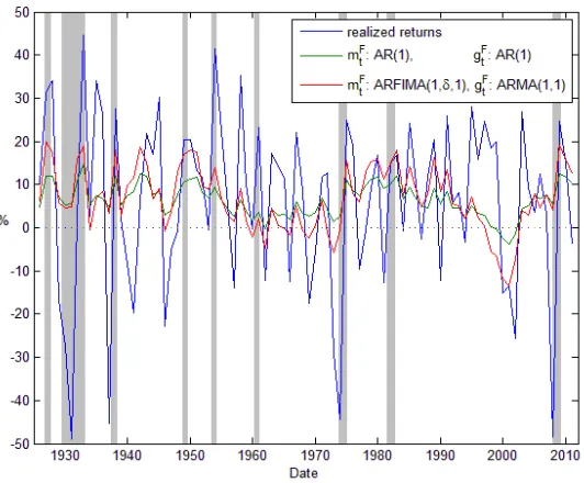
In Figure 2 we plot the time series of realized (blue line) and expected returns as im-plied by the modelsAR(1) AR(1)(green line) andARF IM A(1; ;0) ARM A(1;1)

(red line). The time series for dividend growth (blue line) and expected dividend growth for the AR(1) AR(1) (green line) and ARF IM A(1; ;0) ARM A(1;1)

(red line) are shown in Figure 3. The grey areas denote the NBER recession pe-riods. Since our data is annual, we plotted only recessions that lasted at least 9

months. We can see that the higher variability of expected returns implied by the

series also exhibits a countercyclical pattern.

In order to examine the cyclicality of expected returns and dividend growth we regress a set of macro variables on the …ltered series of expected returns and expected dividend growth. The macro series are growth of real consumption ( Cons), growth of real GDP ( GDP) and growth of industrial production of consumption goods ( IP). The growth of the series is de…ned as the log di¤erence. We chose these vari-ables since they are meaningful indicators of the business cycle. The …ltered series are obtained from the whole available sample of returns, that is1926 2011, however the consumption growth andGDP growth are available only from 1930 and indus-trial production growth only from1940, the regressions are therefore run for those respective periods.15 _{In Table 8 we report the slope coe¢cients with thet statistics}

calculated from the ordinary least squares (OLS) standard errors (reported in small font) and the regression R2_.16 _{In Panel A we report the regression on expected}

returns while the regression on implied dividend growth is reported in PanelB. The results allow us to make a few observations. First, despite the countercyclical nature of both expected returns and expected dividend growth, the latter is a stronger predictor of the business cycle. It is especially visible for predictive regressions of

GDP growth; while the expected returns are not signi…cant and have the slope coe¢cients close to zero, the expected dividend growth have statistically signi…cant slopes at5%level for all models.

series, where theR2 _{value increases from0:13for theAR(1) AR(1)model to0:19}

for theARF IM A(1; ;0) ARM A(1;1)model.

These results suggest that obtaining implied expected returns and dividend growth series can have an important application as leading economic indicators. Particularly more so if the PV model includes a fractional integration component, since this leads to a larger degree of countercyclicality for both the case of expected returns and expected dividend growth as indicated by a largerR2 _statistic.

5

Conclusion

In this paper we show that the long range persistence of the price-dividend ratio ren-ders the simple return forecasting regression considered by Fama and French (1988a) as invalid. Moreover, we argue that in …nite sample the order of integration of the log return series should be approximately the same as that of the …rst di¤erenced price-dividend ratio, which induces negative memory in the return series. We found evidence con…rming this conjecture using semi-parametric estimators; we found that the dividend ratio series is nonstationary but mean reverting with a fractional inte-gration parameter estimate of about0:8, while the return series is characterized by a fractional integration parameter amounting to about 0:2.

We incorporate the fractional integration feature in the PV model using an

ARF IM A time series speci…cation. Using model selection criteria we found that the preferable joint model is the one withARF IM A(1; ;0) expected returns and

Notes

1_{Lettau and Van Nieuwerburgh (2008) explained the strong persistence in the}

price-dividend series as a result of structural breaks (or shifts) in the steady state mean of the economy. They showed that if the shifts are accounted for, then the return forecasting ability of the price-dividend ratio is stable over time. These …nd-ings reinforce the long memory argument in the price-dividend ratio. As showed by Diebold and Inoue (2001), rare structural breaks and long memory are really two sides of the same coin and they cannot be distinguished from each other in …nite samples. On the other hand, Granger and Hyung (2004) established that, if the true series is a long memory process, it is very likely that spurious breaks will be de-tected. Conversely, even if the true process was generated by occasional breaks, the long memory process can successfully reproduce many features of the true series and (under some conditions) can yield better forecasts. Indeed, Lettau and Van Nieuwer-burgh (2008) reported that di¢culties with detecting the breaks in real time makes it hard to forecast stock returns. An alternative explanation of the long memory feature in the aggregate price-dividend ratio could be due to aggregation. Granger (1980) has shown that "integrated series can occur from realistic aggregation situ-ations" (for example: independent series generated by a …rst order autoregressive process can result in a fractionally integrated series when aggregated).

2_{Negative serial correlation in common stock returns at long horizons has indeed}

such long-run return reversals, however, supports the idea that mean reversion can be consistent with the e¢cient functioning of markets as argued by Malkiel (2003).

3_{See also Campbell and Diebold (2009) and references therein.}

4_{Willinger, Taqqu and Teverovsky (1999) found evidence of small degree of long}

range dependence in stock returns. On the other hand, Lo (1991) found no statistical evidence of long memory in stock returns. Lobato and Savin (1998) study rejected the hypothesis of long memory in the levels of returns but found the presence of long memory in squared returns (in line with the …ndings of Ding, Granger and Engle (1993)). Recent studies have reinforced the view that long memory is important to the understanding of asset prices. Bollerslev, Osterrieder, Sizova and Tauchen (2013) estimate a fractionally cointegrated VAR model for returns, objective and risk-neutral volatilities using high-frequency intraday data. Sizova (2013) demonstrates that accounting for long memory in predictive variables is important when considering long-horizon return regressions.

5_{Since the number of lags in the test selected by AIC is0, the test collapses to}

the simple Dickey-Fuller test.

6_{We considered extensions of di¤erent autoregressive and moving average}

or-ders of ARF IM A processes for both the expected returns and expected dividend growth processes and found the ARF IM A(1; m;0) model of expected returns and

ARM A(1;1)model of expected dividend growth to be the most general speci…cation with all coe¢cients signi…cant at the5%level.

7_{See Brockwell and Davis (2009) for details on deriving the moving average}

coef-…cients.

of long memory see Brockwell and Davis (2009) or Palma (2007).

9_{Although monthly or quarterly data would be preferable, we found a strong}

seasonal pattern in the correlogram of dividend growth series at quarterly frequency, which, if not accounted for, invalidates the time series analysis of the dynamics. See also Ang and Bekaert (2007) and Cochrane (2011), appendix. A.1.

10_{Since …rms can pay dividends at di¤erent times of a year, as shown by Cochrane}

(1991), dividends paid early in the year are treated as reinvested at the market rate of return to the end of the year. Van Binsbergen and Koijen (2010) considered the PV model with market reinvested and risk-free rate reinvested strategies and showed that the resulting aggregate dividend growth series are very similar.

11_{The di¤erence between the observed and implied dividend growth is negligible.}

The correlation between these two series amounts to0:9997.

12_{See appendix for details.}

13_{For a more detailed discussion of this argument see Hendry (1995).}

14_TheR2 _{values for annual returns reported in the literature for the long sample,}

starting in 1926 are about3% 9%, see e.g. Campbell, Lo and MacKinlay (1997), ch.7, Goyal and Welch (2003). The price-dividend ratio is generally found to forecast returns better in the second half of the twentieth century until the 1990s, as evidenced by Campbell et al. (1997), Goyal and Welch (2003), Lewellen (2004) and Koijen and Van Nieuwerburgh (2011). Lettau and Van Nieuwerburgh (2008) considered a 30

year rolling sample and foundR2 _{values ranging from close to zero to30%.}

15_{The macro data was obtained from the Federal Reserve Economic Data (FRED),}

16_{In the regressions we did not detect neither heteroskedasticity nor autocorrelation}

References

Andersson, M. K. and Nydahl, S.: 1998, Rational bubbles and fractional alternatives,

Unpublished working paper.

Ang, A. and Bekaert, G.: 2007, Stock return predictability: Is it there?, Review of Financial Studies20(3), 651–707.

Barro, R. J.: 1990, The stock market and investment,Review of Financial Studies

3(1), 115–131.

Bollerslev, T., Osterrieder, D., Sizova, N. and Tauchen, G.: 2013, Risk and return: Long-run relations, fractional cointegration, and return predictability, Journal of Financial Economics108(2), 409–424.

Brockwell, P. J. and Davis, R. A.: 2009,Time series: theory and methods, Springer, second edition.

Campbell, J. Y. and Cochrane, J. H.: 1999, By force of habit: A consumption based explanation of aggregate stock market behavior, Journal of Political Economy

107(2), 205–251.

Campbell, J. Y., Lo, A. W. and MacKinlay, C. A.: 1997, The Econometrics of Financial Markets, Princeton University Press Princeton, NJ.

Campbell, J. Y. and Shiller, R. J.: 1988, The dividend-price ratio and expectations of future dividends and discount factors,Review of Financial Studies1(3), 195– 228.

Campbell, S. D. and Diebold, F. X.: 2009, Stock returns and expected business conditions: Half a century of direct evidence,Journal of Business & Economic Statistics27(2), 266–278.

Chan, N. H. and Palma, W.: 1998, State space modeling of long-memory processes,

Chen, N.-F., Roll, R. and Ross, S. A.: 1986, Economic forces and the stock market,

Journal of Business59(3), 383–403.

Cochrane, J. H.: 1991, Volatility tests and e¢cient markets: A review essay,Journal of Monetary Economics27(3), 463–485.

Cochrane, J. H.: 1999, New facts in …nance,Economic Perspectives(Q III), 36–58. Cochrane, J. H.: 2005,Asset pricing, Princeton University Press, Princeton.

Cochrane, J. H.: 2008a, The dog that did not bark: A defense of return predictability,

Review of Financial Studies21(4), 1533–1575.

Cochrane, J. H.: 2008b, State-space vs. var models for stock returns, Unpublished working paper .

Cochrane, J. H.: 2011, Presidential address: Discount rates, Journal of Finance

66(4), 1047–1108.

De Bondt, W. F. M. and Thaler, R.: 1985, Does the stock market overreact?,Journal of Finance40(3), 793–805.

Dickey, D. A. and Fuller, W. A.: 1979, Distribution of the estimators for autoregres-sive time series with a unit root,Journal of the American Statistical Association

74(366a), 427–431.

Diebold, F. X. and Inoue, A.: 2001, Long memory and regime switching,Journal of Econometrics105(1), 131–159.

Ding, Z., Granger, C. W. J. and Engle, R. F.: 1993, A long memory property of stock market returns and a new model,Journal of Empirical Finance1(1), 83–106. Fama, E. F.: 1990, Stock returns, expected returns, and real activity, Journal of

Finance45(4), 1089–1108.

Fama, E. F. and French, K. R.: 1988a, Dividend yields and expected stock returns,

Journal of Financial Economics22(1), 3–25.

stock prices,Journal of Political Economy96(2), 246–273.

Fama, E. F. and French, K. R.: 1989, Business conditions and expected returns on stocks and bonds, Journal of Financial Economics25(1), 23–49.

Ferson, W. E., Sarkissian, S. and Simin, T. T.: 2003, Spurious regressions in …nancial economics?,Journal of Finance58(4), 1393–1414.

Geweke, J. and Porter-Hudak, S.: 1983, The estimation and application of long memory time series models,Journal of Time Series Analysis 4(4), 221–238. Goyal, A. and Welch, I.: 2003, Predicting the equity premium with dividend ratios,

Management Science49(5), 639–654.

Granger, C. W. J.: 1980, Long memory relationships and the aggregation of dynamic models, Journal of Econometrics14(2), 227–238.

Granger, C. W. J. and Hyung, N.: 2004, Occasional structural breaks and long memory with an application to the s&p 500 absolute stock returns, Journal of Empirical Finance11(3), 399–421.

Granger, C. W. J. and Joyeux, R.: 1980, An introduction to long-memory time series models and fractional di¤erencing,Journal of Time Series Analysis1(1), 15–29. Granger, C. W. J. and Newbold, P.: 1974, Spurious regressions in econometrics,

Journal of Econometrics 2(2), 111–120.

Hamilton, J. D.: 1994,Time series analysis, Princeton University Press, Princeton. Hendry, D. F.: 1995,Dynamic econometrics, Oxford University Press.

Hodrick, R. J.: 1992, Dividend yields and expected stock returns: Alternative proce-dures for inference and measurement,Review of Financial studies5(3), 357–386. Hosking, J. R. M.: 1981, Fractional di¤erencing,Biometrika68(1), 165–176. Koijen, R. S. J. and Van Nieuwerburgh, S.: 2011, Predictability of returns and cash

‡ows,Unpublished working paper.

growth, Journal of Financial Economics76(3), 583–626.

Lettau, M. and Van Nieuwerburgh, S.: 2008, Reconciling the return predictability evidence, Review of Financial Studies21(4), 1607–1652.

Lewellen, J.: 2004, Predicting returns with …nancial ratios, Journal of Financial Economics74(2), 209–235.

Lo, A. W.: 1991, Long-term memory in stock market prices, Econometrica

59(5), 1279–1313.

Lobato, I. N. and Savin, N. E.: 1998, Real and spurious long-memory properties of stock-market data,Journal of Business & Economic Statistics16(3), 261–268. Malkiel, B. G.: 2003, The e¢cient market hypothesis and its critics, Journal of

Economic Perspectives17(1), pp. 59–82.

Mankiw, G. N. and Shapiro, M. D.: 1986, Do we reject too often?: Small sample prop-erties of tests of rational expectations models,Economics Letters20(2), 139–145. Maynard, A. and Phillips, P. C. B.: 2001, Rethinking an old empirical puzzle: econo-metric evidence on the forward discount anomaly,Journal of Applied Economet-rics16(6), 671–708.

Menzly, L., Santos, T. and Veronesi, P.: 2004, Understanding predictability,Journal of Political Economy112(1), 1–47.

Mincer, J. A. and Zarnowitz, V.: 1969, The evaluation of economic forecasts, In Mincer, J. (ed.), Economic Forecasts and Expectations: Analysis of Forecasting

Behavior and Performance, NBER.

Palma, W.: 2007, Long-memory time series: theory and methods, Vol. 662, John Wiley & Sons.

Pástor, L. and Stambaugh, R. F.: 2009, Predictive systems: Living with imperfect predictors,Journal of Finance 64(4), 1583–1628.

and implications,Journal of Financial Economics 22(1), 27–59.

Robinson, P. M.: 1995, Gaussian semiparametric estimation of long range depen-dence,Annals of Statistics23(5), 1630–1661.

Rytchkov, O.: 2012, Filtering out expected dividends and expected returns,Quarterly Journal of Finance2(03), 1–56.

Shimotsu, K.: 2010, Exact local whittle estimation of fractional integration with unknown mean and time trend,Econometric Theory26(02), 501–540.

Sizova, N.: 2013, Long-horizon return regressions with historical volatility and other long-memory variables, Journal of Business & Economic Statistics31(4), 546– 559.

Stambaugh, R. F.: 1986, Bias in regressions with lagged stochastic regressors, Un-published working paper.

Stambaugh, R. F.: 1999, Predictive regressions, Journal of Financial Economics

54(3), 375–421.

Van Binsbergen, J. H. and Koijen, R. S. J.: 2010, Predictive regressions: A present-value approach,Journal of Finance 65(4), 1439–1471.

Welch, I. and Goyal, A.: 2008, A comprehensive look at the empirical performance of equity premium prediction,Review of Financial Studies21(4), 1455–1508. Willinger, W., Taqqu, M. S. and Teverovsky, V.: 1999, Stock market prices and

Appendix A

In this section we discuss the Kalman …ltering procedure and then present the log likelihood function which will subsequently be maximized.

In order to obtain the Kalman equations it is convenient to write the measurement equations in the form where the shocks are lagged relatively to the state vector (see e.g. Brockwell and Davis (2009)). Therefore we de…ne the new state variables

xm;t+1=Cm;tandxg;t+1=Cg;t, so the transition equations are now

xm;t+1=Fxm;t+hm"m;t; (A-1)

xg;t+1=Fxg;t+hg"g;t; (A-2)

and the measurement equations are:

dt= g+w

0

xg;t+"d;t; (A-3)

pdt=A+b0Fxg;t b0Fxm;t+b0hg"g;t b0hm"m;t: (A-4)

In general notation the transition and measurement equations are

xt+1=Fxt+vt; (A-5)

with

xt=

2 6 6 4 xm;t xg;t 3 7 7 5;F=

2 6 6 4 F 0 0 F 3 7 7 5;vt=

2 6 6 4 hm"m;t hg"g;t 3 7 7 5;

yt=

2 6 6 4 dt pdt 3 7 7 5; e=

2 6 6 4 g A 3 7 7

5; W= 2 6 6 4 w0 0 b0

F b0

F

3 7 7 5; zt=

2 6 6 4 "d;t b0

hg"g;t b0

hm"m;t

3 7 7 5;

where0is an in…nite dimensional matrix of zeros. The Kalman recursive equations of the model are:

8 > > > > > > > > > > < > > > > > > > > > > :

t=W tW

0

+R

t=F tW

0

+S

t+1=F tF

0

+Q t t1

0

t

b

xt+1=Fbxt+ t t1 yt e Wxbt

9 > > > > > > > > > > = > > > > > > > > > > ; (A-7) where Q= 2 6 6 4

hgh0g 2g hgh0m mg m g

hmh0g mg m g hmh0m 2m

3 7 7 5; R= 2 6 6 4 2 d b 0

h_{g gd g d} b0

h_{m md m d}

b0

h_{g gd g d} b0

h_{m md m d}(b0

hg)2 2g+ (b

0

hm)2 2m 2b

0

hgb0hm mg m g

3 7 7 5; S= 2 6 6 4

h_{g gd g d} hgb0hg 2g hgb0hm mg m g

h_{m md m d}hmb0hg mg m g hmb0hm 2m

3 7 7 5;

using as initial conditionx1=0:

The log likelihood function is then given by:

`= (2 ) kT =2

T

Q

t=1

det t

1=2

exp 1

2

T

X

t=1

(yt ybt)

0 ₁

j (yt ybt)

!

t adf

0:2046

0:1285 00::94170384 1:5199

p/d ratio returns div.growth GPH

std:err: 10::07632138 00:2138:2313 00::21383738

Robinson

std:err: 00::81171091 00:1091:2154 00::10913479

Shimotsu

std:err: 00::80791078 00:1078:1690 00::10782438

p/d ratio returns div.growth Mean 3:3294 6:1290 1:9898

Std Dev 0:4301 20:0743 14:8599

Skew 0:6154 0:7672 0:1650

Ex. Kurtosis 0:1252 0:4177 0:2310

Min 2:6268 48:8422 30:8588

Max 4:4991 44:6672 44:0666

1st lag Autocorr. 0:9243 0:0164 0:1279

10th lag Autocorr. 0:3983 0:0442 0:0395

Model mt: gt: AR(1) AR(1) AR(1)

ARM A(1;1)

ARF IM A(1; ;0)

AR(1)

ARF IM A(1; ;0)

ARM A(1;1)

m std:err

0:0644

0:0159 00::06340169 00::06650159 00::06590182

m std:err

0:8321

0:0747 00::82540719 00::89170498 00::88400510

std:err 00::13683269 00::13032929

g std:err

0:0179

0:0145 00::01700151 00::01800157 00::01760179

g std:err

0:6050

0:2392 00::08618861 00:2156:5348 00::10098714

std:err 00::58742229 00::57642360

m std:err

0:0322

0:0131 00::03690141 00::06610158 00::06840179

g std:err

0:0599

0:0200 00::06510167 00::07190191 00::07310174

d

std:err 00::12930145 00::12960113 00::12680116 00::12860115 mg

std:err

0:8410

0:0854 00::90980684 00::86640677 00::91830574

Model

mt:

gt:

AR(1)

AR(1)

AR(1)

ARM A(1;1)

ARF IM A(1; ;0)

AR(1)

ARF IM A(1; ;0)

ARM A(1;1)

k 8 9 9 10

LR

p value 20::70750999 20::67161022 40::84180888

AIC 164:2585 164:9660 164:9302 165:1004

BIC 139:0786 136:6386 136:6027 133:6254

(mt) 3:8189 4:2736 7:2302 7:4888

(gt) 5:1369 5:4733 5:8259 6:0329

corr(mt; gt) 0:1239 0:3043 0:3817 0:4986

R2

r 0:1321 0:1443 0:2060 0:2058 R2

d 0:3166 0:3200 0:3763 0:3577

Model mt: gt: AR(1) AR(1) AR(1)

ARM A(1;1)

ARF IM A(1; ;0)

AR(1)

ARF IM A(1; ;0)

ARM A(1;1)

Panel A:rt+1= + mFt +ut

std:err: 00::03820869 00:0352:0724 00::02630252 00::02610227

std:err:

2:3248

0:5144 20::09244589 10::29392680 10::23942593

t val:(H0: = 0) 2:2777 2:0558 0:9582 0:8685

t val:(H0: = 1) 2:5755 2:3806 1:0964 0:9232

F (H0: = 0; = 1)

p value

3:3246

0:0408 20::84250639 00::64285284 00::48206193

F test[AR(1) AR(2)]

p value

2:8533

0:0634 30::24630440 30::10440502 30::03330536

Panel B: dt+1= + gFt +ut

std:err: 00::05850232 00::05440229 00::05000227 00::04740225

std:err:

0:1468

0:4261 00::36853982 00::56973708 00::68553553

t val:(H0: = 0) 2:5202 2:3713 2:2026 2:1077

t val:(H0: = 1) 2:0024 1:5860 1:1605 0:8852

F (H0: = 0; = 1)

p value

7:2104

0:0013 50::26100070 70::32220012 40::76470110

F test[AR(1) AR(2)]

p value

3:7835

0:0269 10::96511468 20::56210834 10::48142334

Table 6: Results of the Mincer-Zarnowitz (1969) regressions for real returns (Panel A) and dividend growth (Panel B) for di¤erent present-value models. In Panel A we regress returns on a constant and the …ltered values of expected returns. In the …rst two lines we report the estimated coe¢cients with their standard errors and in the following two lines the t-statistic for the null hypothesis of unbiased and consistent forecasts, that isH0: = 0 andH0: = 1 . In the next line we report theF test

of the joint null hypothesis H0 : = 0 and = 1 with the p-values. The last line

Model

mt:

gt:

AR(1)

AR(1)

AR(1)

ARM A(1;1)

ARF IM A(1; ;0)

AR(1)

ARF IM A(1; ;0)

ARM A(1;1)

Panel A: In-sample forecast

R2

r 0:0310 0:0297 0:0948 0:0914 R2

d 0:1099 0:1535 0:1315 0:1659

Panel B: Fixed point estimation forecast

R2

r 0:0311 0:0396 0:0433 0:0359 R2

d 0:1015 0:1258 0:1080 0:1304

Panel C: Recursive estimation forecast

R2

r 0:0209 0:0295 0:0183 0:0083 R2

d 0:0733 0:1005 0:0883 0:1058

Model mt: gt: AR(1) AR(1) AR(1)

ARM A(1;1)

ARF IM A(1; ;0)

AR(1)

ARF IM A(1; ;0)

ARM A(1;1)

Panel A:

Const+1= + mFt +u

t value

0:2666

3:3171 03::24603988 03::15025959 03::14395393

R2 _{0:1236 0:1290 0:1422 0:1384}

GDPt+1= + mFt +u

t value

0:0062

0:0437 00::01220956 00::02393225 00::02223088

R2 _{0:0000 0:0001 0:0013 0:0012}

IPt+1= + mFt +u

t value

0:2785

2:0031 02::25920630 02::15351268 02::14740990

R2 _{0:0557 0:0589 0:0624 0:0608}

Panel B:

Const+1= + gtF+u

t value

0:2063

3:4067 03::22059450 04::20820264 04::21563383

R2 _{0:1295 0:1663 0:1721 0:1944}

GDPt+1= + gFt +u

t value

0:2108

2:0274 02::20841308 02::18430250 02::17850118

R2 _{0:0501 0:0550 0:0499 0:0493}

IPt+1= + gtF+u

t value

0:3330

3:1928 03::34374493 03::31585102 03::31966055

R2 _{0:1304 0:1489 0:1534 0:1605}

Figure 2: Realized returns (blue line) and expected returns as implied by the models

Figure 3: Realized dividend growth (blue line) and expected dividend growth as im-plied by the modelsAR(1) AR(1)(green line) andARF IM A(1; ;0) ARM A(1;1)