A strategic model for network formation
Atabati, Omid and Farzad, Babak
University of Calgary, Brock University
1 November 2014
Online at
https://mpra.ub.uni-muenchen.de/62529/
Omid Atabati1 and Babak Farzad2
1
Department of Economics, University of Calgary
2
Department of Mathematics, Brock University
Abstract. We study the dynamics of a game-theoretic network formation model that yields large-scale small-world networks. So far, mostly stochastic frameworks have been utilized to explain the emergence of these networks. On the other hand, it is natural to seek for game-theoretic network formation models in which links are formed due to strate-gic behaviors of individuals, rather than based on probabilities. Inspired by Even-Dar and Kearns’ model [8], we consider a more realistic framework in which the cost of establishing each link is dynamically determined during the course of the game. Moreover, players are allowed to put transfer payments on the formation and maintenance of links. Also, they must pay a maintenance cost to sustain their direct links during the game. We show that there is a small diameter of at most 4 in the general set of equilibrium networks in our model. We achieved an economic mechanism and its dynamic process for individuals which firstly; unlike the earlier model, the outcomes of players’ interactions or the equilibrium networks are guaranteed to exist. Furthermore, these networks coincide with the out-come of pairwise Nash equilibrium in network formation. Secondly; it generates large-scale networks that have a rational and strategic microfoundation and demonstrate the main characterization of small degree of separation in real-life social networks. Furthermore, we provide a network formation simulation that generates small-world networks.
Keywords: network formation, linking game with transfer payments, pairwise stability, pairwise Nash equilibrium, small-world phenomenon
JEL classifications:D85, C79
1
Introduction
In recent years, networks have been extensively studied mostly in terms of their structure, but also their formation and dynamics. Structural characteristics of various networks, which emerge from disciplines, such as economics, computer science, sociology, biology and physics, have been
⋆
A revised version has been accepted in the journal of Computational Social Networks. Suggested citation:
investigated. Many of these networks, in spite of their different origins, indicate large common-alities among their key structural properties, such as small diameter, high clustering coefficient, and heavy-tailed degree distribution which are often quantified by power-law probability distribu-tions. Hence, it is an exciting challenge to study network formation models capable of explaining how and why these structural commonalities both occur and evolve. The series of experiments by Milgram in the 1960s [17] were among the pioneering works that quantified thesmall-world phenomenon3and introduced the “six degree of separation”. Recent experiments [6] showed that
today’s online social networks such as Facebook indicate that the degree of separation (for almost any two individuals in a given database) must be even smaller than 4.
Thesmall-world model by Watts and Strogatz [20] was one of the first models that generates networks with small diameter. This work followed by Kleinberg’s stochastic model [16] that was located in a grid graph. It introduced a process that adds links with distancedto the grid with a probability proportional to 1/dα. These models, however, can not be applicable when there
is a strategical purpose in players’ making or losing their connections. In these cases, players, which are represented by vertices, strategically establish and sever their connections to obtain an advantageous position in their social network. Hence, we refer to a class of game-theoretic network formation, also known as strategic network formation (See [7, 12] for comprehensive surveys). Models in this class are in their early efforts. They generally assume that players make connections based on a utility maximization and treat the network as the equilibrium result of the strategic interactions among players.
1.1 Our contribution
Our game-theoretic network formation model is mainly inspired by Even-Dar and Kearns (EK model) [8]. In their model, players (i.e., vertices) seek to minimize their collective distances to all other players. The network formation starts from a seed grid. Also, the cost of establishing each link in this model is considered to be the grid distance between the endpoint players of that link to the power of α, which is the parameter of the model. Hence, their model uses a
fixed link-pricingfor each link. Both link creation and link severance are considered unilateral by players. In addition, the equilibrium is defined in terms oflink stability: no players benefit from altering a single link in their link decisions. The EK model achieves small diameter link stable networks within the threshold ofα= 2. However, they faced an unbounded diameter that grows with the number of players, whenα >2.
We define three types of costs for links: (i) the link-price, (ii) the maintenance cost, and (iii) the transfer payment. The link-price pij is the price of establishing link ij. Only the initiator
of connection would bear its payment. It is a one-time charge when establishing the link. We introduce a new viewpoint to this game that better echoes with reality by constructing adynamic
3
link-pricing. When characterizing the formation of a network, the involved dynamics is a crucial and determining element. We aim to effectuate the impact of this dynamics in our model with the revised link-pricing. We update the used distances of each pair of players in the related link-prices from the current network rather than sticking with the initial grid distances.
In addition, we introduce maintenance costs to make the model more real where a player can give up her payment and sever her connection, if she’ll be better off by doing so. Also, it is reasonable to assume that refunding the link-prices may not be possible in lots of real-world scenarios. Hence, maintenance costs make the link severance scenario well-defined. In our model, player i is charged for all of its incident links by considering recurring maintenance costs cij.
In other words, for each decision made in the game, players should take the maintenance cost of their incident links into their consideration. Lastly, we allow individuals to put transfer or side payments on their links. Transfers are a sort of communication between players for their connections. In fact, without transfer payments, many agreements on these connections would simply never exist.
We use the myopic notion of Pairwise Stability with direct and indirect transfers (P St)4as our
equilibrium notion. This notion has the advantage of being compatible with the cooperative and bilateral nature of link formation. Moreover, the pairwise stability has the desirable simplicity required for analyzing players’ behaviors under this notion.5
On the other hand, due to the bilateral agreement for any link formation, the typical notion of Nash equilibria has some drawbacks in terms of coordination failures; e.g. an empty network is always a Nash equilibrium. In other words, Nash equilibria networks can contain some mutually beneficial link(s) that are left aside. To solve this coordination problem when employing Nash equilibria, the notion of pairwise Nash stability6was introduced. Pairwise Nash Stable (P N St)
networks are at the intersection of the set of Nash equilibrium networks and the set of pairwise stable networks.
In this paper, we not only guarantee the existence of pairwise stable networks, but also demonstrate that, in our model, the set of pairwise stable networks coincide with the set of pairwise Nash stable networks. Finally, we show that the general set of equilibrium networks exhibits a short diameter of at most 4. The rest of this paper is organized as follows. In Section 2, we explain the required preliminaries and provide the setup of our model. Section 3 contains an analysis and extension to the EK model. We then provide the main results for our grid-based
4
The pairwise stability is the major notion of stability that assumes myopic players and has been studied in related literature. In a linking game with transfers, it was first introduced as an extension in [15] and then developed in [2, 3].
5
Computing the best responses of players in Nash equilibria within some similar models [18, 9] are proved to be NP-hard.
6
model with the dynamic link-pricing and transfer payments in Section 4. In Section 5, we present the outcome of a network formation simulation that we carried out.
2
Preliminaries
The network and players. Let N = {1, ..., n} be the set of n players forming a network G. Network G is undirected and includes a list of pairs of players who are linked to each other. Linkij ∈Gindicates that player iand player j are linked in G. Let GN denote the complete
network. The setG =
G⊆GN consists of all possible networks onN. We define networkG0
to be the starting network of the game, which is also called theseed network. The set of playeri’s neighbors inGis Ni(G) ={j|ij ∈G}. Similarly,Li(G) ={ij∈G|j∈ Ni(G)} denotes the set
of links, which are incident with playeriinG. Ifl is a subset ofLi(G), thenG−lis the network
resulted by removing the existing links in the setlfromG. Similarly, ifl={ij|j /∈ Ni(G), j6=i},
then the networkG+l is obtained by adding the links in setl toG.
The utility of network G for player i is given by a function ui : G → R+. Let u denote
the vector of utility functionsu= (u1, ..., un). So, u: G → RN. Also, the value of a network,
v(G), is the summation of all players’ utilities in the network G; i.e., v(G) = Pn
i=1ui(G). For
any network G and any subset li(G)⊆ Li(G), the marginal utility for a player i and a set of
linksli(G) is denoted bymui(G, li(G)) =ui(G)−ui(G−li(G)).
Strategies; transfer payments.Each player i∈N announces an action vector of transfer pay-mentti∈Rn(n−1)/2. The entries in this vector indicate the transfer payment that playerioffers (to pay) or demands (to gain) on the linkjk. Ifi∈ {j, k}, then we call it adirecttransfer payment. Otherwise, it is called an indirect transfer payment. Typically, individuals can make demands (negative transfers) or offers (non-negative transfers) on their direct connections. However, they can only make offers (and not demands) on the indirect transfer payments.7In addition, a linkjk
is formed if and only ifP
i∈Ntijk≥0. Thus, the profile of strategies or the announced vectors of
transfer payments for all players is defined:t= (t1, ...,tn). Consequently, the networkG, which is formed by this profile of strategiest, can be denoted as follows:
G(t) ={jk|P
i∈Ntijk≥0,wherej, k∈N}.
The payoff function. Thedistance between a pair of playersiandjinG, denoted bydG(i, j),
is defined as the length of a shortest path betweeniandj inG. Similar to the EK model, players seek to minimize their total distances to all players. This benefit would be considered for each player with respect to the networkGand links benefit both endpoints.8The link-price is defined
7
This assumption is reasonable in our framework, since the formation of other links cannot hurt the utility of non-involved players with respect to the distance-based structure of our utility function in (1).
8
to bepij =dG(i, j)αforα >0. The link-price function is non-decreasing and follows Kleinberg’s
stochastic model. Also, function cij denotes the maintenance cost for the link ij. The utility function of playeri is the negative of her total distances and links expenses and is defined as follows:
ui(G(t)) =−
X
j∈N
dG(t)(i, j)−
X
j∈Ni
cij−
X
j∈Si
pij−
X
jk∈G(t)
tijk, (1)
whereSi is a subset ofi’s neighbors whose links toiare initiated byiin the network formation. The dynamic process. The following notion is stated from [13] that motivates the desired dynamics for our analysis.
Definition 1 An improving path represents a sequence of changes from one network to another. The changes can emerge when individuals create or sever a single link based on the improvement in the resulting network relative to the current network.
In each round of the game, one player adapts her strategy with respect to the current state of the network. We assume a random meeting mechanism for vertices (randomly choosing a pair of players), but we start with a seed network instead of an empty network [19, 14]. If two networks
Gand G′ differ in exactly one link, they are said to be adjacent networks. Also, if there exists an improving path fromGto G′, thenG′ defeats G.
The equilibrium strategies.In every equilibrium profile of strategiest∗, there is no excess in the offer of transfer payments. A transfer paymentt∗i
ij is negative, if and only if maintaining the
existing link ij is not beneficial for i. In other words,i’s utility from network Gis smaller that her utility from network G−ij. We refer to this difference as a utility gap. Player i can only use a transfer payment equal to her utility gap. Hence, for an equilibrium profile of strategiest∗i
jk
that forms equilibrium networkG,
G(t∗) ={jk|P
i∈Nt
∗i
jk= 0, j, k∈N}.
We would like to indicate that other generalization of transfers’ distribution among players are not among the main focuses of this paper.9
Definitions of equilibrium notions:
Definition 2 A network Gis Pairwise Stable with transfers (P St) with respect to a profile of utility functions uand a profile of strategiestthat creates network Gif
(a) ij∈G =⇒ ui(G)≥ui(G−ij)as well as uj(G)≥uj(G−ij),
9
(b) ij /∈G =⇒ ui(G)≥ui(G+ij) as well asuj(G)≥uj(G+ij).
Also,P St(u) denotes the family of pairwise stable networks with transfers.
A pure strategy profilet∗= (t∗1, ...,t∗n) forms aNash equilibrium in the linking game with transfers if ui(G(ti,t∗−i)) ≤ ui(G(t∗)) holds for all i ∈ N and all ti ∈ Ti, where t∗−i is the
equilibrium strategy for all players other thani, andTi is the set of all available strategies fori.
We can also indicate that in the context of network formation, a networkG is Nash stable iff
∀i∈N, and∀li(G)⊆ Li(G):ui(G)≥ui(G−li(G)).
Definition 3 A pure strategy profilet∗= (t∗1, ...,t∗n)forms a pairwise Nash equilibrium in the
linking game with transfers if
1. it is a Nash equilibrium, and
2. there does not exist any ij /∈G(t∗), andt∈T such that
(a) ui(G(tiij,tjij,t∗−ij))≥ui(G(t∗)), (b) uj(G(tiij,t
j ij,t
∗
−ij))≥uj(G(t∗)), and (c) at least one of (1) or (2) holds strictly,
wheret∗−
[image:7.595.284.349.419.491.2]ij includes all players’ strategies int∗ except player i.
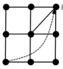
Fig. 1.An example of a sub-network from networkGduring the dynamic process
A tutorial example. Suppose that Figure 1 shows a sub-network of a network G that is obtained through an improving path. Also, assume that playericonsiders establishing a link to playerj in the next random meeting. Fur this example, let assumeα= 2 andcij = 10 for alli
andj. Furthermore,Bi(G+ij, ij) =−Pk6=i(dG+ij(i, k)−dG(i, k)) defines the benefit of reduced
distances in the whole networkGthat playeriis received after adding linkij toG. We assume thatBi(G+ij, ij) = 30 andBj(G+ij, ij) = 5 in this example.
According to the dynamic link-pricing,pij = 32= 9. First, we can verify that playerihas an
incentive to buy linkij, as Bi(G+ij, ij) = 30≥9 + 10 = 19. However, there is no advantage
for player j in this linking, as Bj(G+ij, ij) = 5 <10. Therefore, player j must demand the
the transfer payment ti
ij = 10−5 = 5 to player j, since creating ij is still beneficial for i, as
30≥5 + 19 = 24.Consequently, linkij can be added toGand networkG′ is achieved along the improving path of game. The network formation continues until a pairwise stable network with transfers is reached. Note that we can also consider the indirect transfers that other players may offer for this linkage, which is not stated in this example for simplicity.
3
Fixed link-pricing model
In this section, we study the EK model [8] and consider an extension to this model. This also helps us to provide some insights regarding our results in Section 4.
3.1 The presence of cycles
The EK model takes a√n×√ngrid as its seed network. It defines the link-pricepij =dG0(i, j)
α
forα >0 and defines dG0(i, j) to be the grid distance ofi andj. Consequently, the link prices
are fixed during the course of the game. Furthermore, this model defines the set si∈ {0,1}n−1
to be the action set of playerisuch thatsij is one when playericreates a link to playerj. Also,
each link benefits both endpoints andsij= 1 iffsji= 1. The utility function for playeri∈N is
ui(G(s)) =−Pj6=idG0(i, j)− P
j∈Nipij.
In the EK model, link creation is unilateral. Moreover, creation of a link only requires the agreement of at least one of the endpoint players of the link. This is in contrast to our model in which the presence of each link needs the consent of both players. Also, there is no transfer payment and maintenance cost in this model. Players can receive a refund of the link-prices given the severance of links. This model uses the notion of link stability, where link stable networks are immune against unilateral creation or severance of a single link by each player.
A problem that can arise in this model concerns the fact that the network formation may not converge to a link stable network. In other words, there exists the possibility for the formation of cycles in the evolving networks during this network formation model, as it is defined in the following.
Definition 4 A cycle C is a set of networks (G1, ..., Gk) such that for any pair of networks
Gi, Gj ∈ C, there exists an improving path connecting Gi to Gj. In addition, a cycle C is a closed cycle, if for all networks G ∈ C, there does not exist an improving path leading to a networkG′ /
∈C.
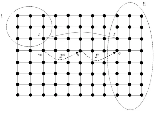
Fig. 2.In this example, the game may not converge to a link stable graph.
Consider the following grid-based example shown in Figure 2. In this example, we can observe the formation of a cycle in the game.
Assume that 48 < 3α < 49. First, it is easy to verify that player s has an incentive to
create linkst. Now a cycle of strategical updates may be formed as follows. Player usaves 57 in
Pn
i=1dG(s)(u, vi) as it can be verified that the distance touof 9 players in area i is reduced by 1
and the distance touof 24 players in area ii is reduced by 2. So, (I) playeruhas an incentive to buy linkuv, aspuv=dG0(u, v)
α= 3α<9 + 48 = 57. Then with similar observations, it can be
seen that the following strategical changes will be made in this order. (II) playerwbuys linkwu
aspwu=dG0(w, u)
α = 3α<49. (III) playeruis no longer willing to maintain link uv, as with
existing linkwu, it has a benefit of only 48. Therefore,ureturns the linkuv. (IV) playerwhas no incentive to retain linkwu, as with the removal of link uv, it has a benefit of only 34. So, w
returns the linkwu. Thus, a cycle of steps (I) to (IV) may be formed and the game does not converge to stability. The example can be expanded to a large-scale grid as well. We note that playerw, by establishingwu, creates a negative externality foru. Since it causes a reduction in playeru’s utility,udecides to severuv that in overall leads to the formation of a cycle.
3.2 Forbidding link severance
In this model, players should be allowed to sever only those links that they themselves have purchased. However, this issue is not clear in the notion of link stability.10Let assume an extension
of EK model with forbidding severing links. Forbidding players to sever their links, although
10
limits the applicability of model, makes the convergence of equilibrium networks possible for the network formation.
Proposition 1 Under the assumption of forbidding link severance in the EK model, the conver-gence of network formation to link stability is guaranteed.
Proof. When there is no link severance, the existence of negative externalities for players is ruled out. In other words, there is no player whose utility can be hurt during the game. Thus, the total value of the network is increased by each change during the dynamic process. This points to theexact pairwise monotonicity, introduced by Jackson and Watts [13], which guarantees the existence of stable networks. The proof of Theorem 1 can be adapted to imply Proposition 1.
4
Dynamic link-pricing model with transfer payments
4.1 Existence of pairwise stable network with transfers
In all game-theoretic problems, one of the primary questions concerns the existence of equilibria or stable states. This question in the framework of network formation is translated to the existence of pairwise stable networks and have been first addressed by Jackson and Watts [13]. We show that their arguments can be extended and adapted in our model. As a result, we guarantee the existence of pairwise stable network with transfers in our model.
While improving paths that start from a seed network may end in an equilibrium network, it is also possible to find the formation of cycles as the result of an improving path. Jackson and Watts showed that in any network formation model there exists either a pairwise stable network or a closed cycle. Their argument is based on the fact that a network is pairwise stable if and only if it does not lie on an improving path to any other network. We provide the following lemma and refer to the work of Jackson and Watts [13] for its proof, where the exact arguments can be applied for the notion of P St in our model.
Lemma 1 In the network formation model with transfer payments, there exists either an equi-librium network from P St(u)or a closed cycle of networks.
Theorem 1 In the linking game with direct and indirect transfers given the utility function in
(1),
(a) there are no cycles,
(b) there exists at least one pairwise stable network(P St(u)).
andGandG′are adjacent.11We can briefly argue that our linking game satisfies this condition.
Since the direct and indirect transfer payments between players prevent the situations, where a player’s utility can get hurt by actions (link addition or deletion) of others. In fact, this is one of the main function of transfers. Therefore, the value of networks through each improving path must be increased. Conversely, if G and G′ are adjacent in an improving path such that
v(G′)> v(G),G′ must defeat G, where Gis a network in the cycle.
Now, since there are finitely many networks that can be reached through the dynamic process, if there is a cycle, then the exact pairwise monotonicity of our linking game impliesv(G)> v(G); contradiction. Ruling out the existence of cycles along with Lemma 1 guarantees the existence of at least one pairwise stable network with transfer payments.
4.2 Strictly pairwise stability
Now, we show that given the utility functionu(.) in (1), the family of networks inP St(u) satisfies
the notion of strictly pairwise stability. It is first described by Chakrabarti and Gilles [5], which is a variation of pairwise stability.
Definition 5 A network Gisstrictly pairwise stableforu, if
(a) ∀i∈N and∀li(G)⊆ Li(G),ui(G)≥ui(G−li(G),
(b) ∀i∈N,ij /∈Gimpliesui(G+ij)< ui(G)as well as uj(G+ij)< uj(G).
In order to progress our argument, we need to provide the following definition and lemma.
Definition 6 Let α≥0. A utility functionu(.)isα-submodular in own current linksonA ⊆ G
if∀i∈N, G∈ A, andli(G)⊆ Li(G), it holds that
mui(G, li(G))≥αPij∈li(G)mui(G, ij).
The caseα= 1 corresponds to submodularity, also called superadditivity in [2].
Lemma 2 The utility defined in (1)is submodular in own current links.
Proof. The proof is inspired by the arguments in [10]. First, we show the related inequality in Definition 6 holds for the case when the subset li(G) consists of two distinct links ij and ik,
which is indicated in the below inequality.
mui(G, ij+ik)≥mui(G, ij) +mui(G, ik) (2)
If we consider any player such asmin networkG, the distance betweeniandm (dG(i, m))
contributes to the distance expenses ini’s utility. It is important to note that removing any link
11
such as ij or ikfrom the network Gcannot decrease this distance, however if the removed link belongs to the shortest path betweeniandm inG, then the distance would be increased. This argument can be extended to the severance of two links such asij andikfromG.
dG(i, m)≤dG−ij(i, m)≤dG−ij−ik(i, m) (3)
dG(i, m)≤dG−ik(i, m)≤dG−ij−ik(i, m) (4)
In computing the marginal utilities of networksG−ik, G−ij, and G−ij−ik, we should note that the link-prices of removed links cannot be refunded for playeri.
mui(G, ij) =−
X
m6=i
(dG(i, m)−dG−ij(i, m))−cij−tiij (5)
mui(G, ik) =−
X
m6=i
(dG(i, m)−dG−ik(i, m))−cik−tiik (6)
mui(G, ij+ik) =−
X
m6=i
(dG(i, m)−dG−ij−ik(i, m))−cij−cik−tiij−tiik (7)
According to Inequalities (3) and (4), we can simply imply the Inequality (2). Finally, we can easily extend this argument for any subset of linksli(G).
Proposition 2 Given the utility functionsu(.)defined in (1),P St(u) =P⋆(u).
Proof. According to the definitions, it can be derived that P⋆(u)
⊆P St(u). We further prove
that P St(u)
⊆ P⋆(u).
LetG∈P St(u), then for any link ij /
∈ G, neither player i norj can benefit from creating linkij. This is one of the impact of allowing players to put transfer payments on the links. Thus, pairwise stable networks with transfers satisfy the second condition in the Definition 5. Further, we know that ∀i∈N, and∀j ∈li(G),ui(G−ij)≤ui(G). Let assume there are k links in the
subset li(G). Hence, Pij∈li(G)ui(G−ij)≤(k)ui(G). On the other hand, based on Lemma 2,
P
ij∈li(G)mui(G, ij)≤mui(G, li(G)). This implies
(k)ui(G)−
X
ij∈li(G)
ui(G−ij)≤ui(G)−ui(G−li(G)). (8)
Since the left-hand side of Inequality (8) is positive, the expression in the right-hand side must be positive too. So, this proves the first condition in the Definition 5 for the networks in
4.3 Convergence to pairwise Nash stability
Calv´o-Armengol and Ilkili¸c [4] show the equivalency of pairwise stable networks and pairwise Nash stable networks, given a utility function that isα-submodular. It targets the simple obser-vation that given aα-submodular utility function, if a player does not benefit from severing any single link, then she does not benefit from cutting any subset of links simultaneously as well. A similar argument can be adapted to our linking game with transfers as well. So, we provide the following proposition without proof.
Proposition 3 Given a profile of utility functions u in (1) in a linking game with transfers,
P St(u) =P N St(u).
4.4 Small diameter in equilibrium networks
We take a large-scale √n×√n grid as the seed network in this model. In order to prove the main result for the diameter of the equilibrium networks, we provide the following lemmas.
LetTG(t)(i, j) be the set of players that use linkij in their unique shortest paths toi in the
networkG(t) :TG(t)(i, j) ={k∈N |dG′(t)(i, k)> dG(t)(i, k)}, whereG′ =G−ij.
Lemma 3 Let G(t) be an equilibrium network and i, j ∈N be an arbitrary pair of players in
this network. Ifij /∈G(t)then|TG(t)(i, j)|< dG(t)(i, j)
α+c ij+tiij
dG(t)(i, j)−1
.
Proof. Sinceiandj are not linked in the equilibrium network, the benefit of establishingij has to be less than its linking costs foriand j. On the other hand,TG(t)(i, j) represents the set of
players that creates a part of this benefit by reducing the distancedG(t)(i, j) betweeniandjto
1. Hence, we can state that payingdG(t)(i, j)α+cij+tiij, which is necessary for establishingij,
cannot be beneficial for playeri. As a result,|TG(t)(i, j)|(dG(t)(i, j)−1)< dG(t)(i, j)α+cij+tiij.
Remark 1 For any i, j∈N,cji can be noted as an upper bound for the transfer payment tiij. Hence, ifc= max∀i,j∈N(cjk), it is an upper bound for any direct transfer payment in the network.
Lemma 4 In any equilibrium network G(t), for any playeri∈N,
letSd
i ={k∈N|dG(t)(i, k)≤d}. Then,|Sdi|(1 +
dα+ 2c
d−1 )≥n, wherec = max∀i,j∈N(cij).
Proof. The set Sd
i consists of players in the neighborhood of i within a distance at most d.
Furthermore, for each of these players such as k in the set Sd
i, according to Lemma 3, we
consider the setTG(t)(i, k). All players outside of this set should use one of players such askin
their shortest path toi. As a result, we can cover all players outside the setSd
setTG(t)(i, k) toifor all players in setSid. By doing so, an upper bound of|TG(t)(i, k)||Sid|+|Sid|
for the number players in network (n) is achieved.
In order to obtain an upper bound for the setTG(t)(i, k) in wide range of different possible
choices for i and k, we define c to be the maximum maintenance cost for all possible links in network. According to Remark 1, this is an upper bound for all the possible direct transfer payments as well. Hence,|TG(t)(i, k)|≤
dα+ 2c
d−1 . By substituting the upper bounds ofTG(t)(i, k) andSd
i in |TG(t)(i, k)||Sid|+|Sid|≥n, the desired inequality can be achieved.
Lemma 5 shows an upper bound for the set|S2
i|.
Lemma 5 |S2
i|≤ ∆α+ 2c
.
k
∆−h1 +h2(g1+ 2) +h3(2f1 +f2 + 3)
, where ∆ is the
diameter of any equilibrium network G(t), and 0 ≤ k, fi, gi, hi ≤ 1 denote some fractions of
players in the setS2
i based on their reduced distances to playeriwhen forming the linkij. Also,
f1+f2+f3=g1+g2=h1+h2+h3= 1.
Proof. LetGbe an arbitrary instance from the set of equilibrium networks in our model, which are the set of pairwise stable networks with transfer (G ∈ P St(u)), given the utility function
u(.) in (1). Also, lettbe the the profile of strategies for players that formsG. Further, assume that the largest distance between any two players (or diameter) in networkGexists between two players i and j. We denote ∆ to be the size this distance. Note that the pair ofi andj is not necessarily unique.
Based on the stable state, we can imply that creationij is not beneficial for neither i nor
j. If j wants to establish a link to i,|S2
i| is a lower bound for the j’s benefit that comes from
the reduced distances to players in S2
i. This set includes iitself and two subsets of players that
are in distance 1 (type 1) and 2 (type 2) fromi. First, letk represents players inS2
i such that
their distances toj can be reduced by addingij, as a fraction with respect to all players in|S2
i|.
Moreover, let h1 represents player i itself as a fraction with respect to all players in |S2i|. By
establishingij,j’s distance toi reduced by ∆−1.
Furthermore, let h2 and h3 represent the fractions of the number of type 1 players and
type 2 players, respectively, in S2
i. Their reduced distances for j is computed according to the
initial distances of these two types of players in S2
i from j. Among the type 1 players, there
are two subsets of players that g1 andg2 are their fractions with distance of ∆−1 and ∆ from
j, respectively. Furthermore, in type 2 players, there are three subsets of players in terms of their distance from j with fractions of f1, f2, f3 that are in distance of ∆−2,∆−1,∆ from j,
respectively.
Proof. Based on our arguments in Lemma 4 and Lemma 5, we can state that
n≤(1 + 2α+ 2c)(∆α+ 2c).k
∆−h1+h2(g1+ 2) +h3(2f1+f2+ 3)
. (9)
For sufficiently large network, when the diameter is greater than⌊h1+h2(g1+ 2) +h3(2f1+
f2+ 3)⌋, it contradicts Inequality (9). Clearly we can specify that 3 ≤2f1+f2+ 3 ≤ 5 and
2≤g1+ 2≤3. Thus in this case, the upper bound for the diameter is the weighted average of 1,
2f1+f2+ 3 andg1+ 2 and it is surely smaller than 5. Therefor, diameter cannot be bigger than
4 for any choice of parameters. However, we cannot have the same claim for smaller diameter and rule out their possibility.
5
Simulations
We carried out a set of simulations that improves the EK model by implementing the dynamic link-pricing and a fixed maintenance costc. These simulations generate networks that show (i) a small diameter of at most 4, (ii) a high clustering coefficient (with respect to edge density), and (iii) a power-law degree distribution. The dynamical simulations are implemented on a grid with
n≈1000. At each iteration of the dynamic process, two playersiandj are chosen uniformly at random. Then, with probability 1/2 playericonsiders establishing a link toj(ifij /∈G) and with probability 1/2 she considers severing her link toj(ifij∈G). Note that these considerations are such that in each random meeting, the decision for adding (or removing) a link is implemented based on the corresponded benefit and cost to that link with respect to the current state of the evolved network. We used the notion of link stability. In this set of simulations, we aim to indicate our improvements and extension on the EK model in order to generate small-world networks. Note that by using the dynamic link-prices, the emergence of a small diameter of at most 4 in link stable networks are directly implied similarly by our argument in Section 4.4.12
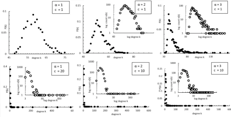
In many instances of our simulations, it can be seen as in Fugure 3 that the degree distribution is a good estimation for the power-law degree distributions in the real-life social networks. Fig-ures 3 shows the impact of parameterscandαon the degree distributions of resulting networks. The larger plots are the distributions where their vertical axis is the probability for degrees and their horizontal axis determines different values for the degree of nodes. The smaller plots are the log-log plots of these distributions. Their vertical axis are the logarithm of the number or the frequency for nodes with different values for their degree. Moreover, the appearance of few high degree nodes represents the few hubs in these networks.
12
Figure 4 demonstrates the clustered structure of the link stable networks: a high average clustering coefficient is present in all instances after increasing the maintenance cost fromc= 1. The high clustering in these networks can be highlighted by pointing out their small edge-density in the range from 0.007 for the network withc= 50,α= 5 to 0.069 for the network withc= 1 andα= 1. The diameter in all instances was either 3 or 4 as expected.
[image:16.595.152.415.455.655.2]Fig. 3. Degree distributions.Structural properties of generated networks in the simulations.
References
1. M. Bayati, C. Borgs, J. Chayes, Y. Kanoria, and A. Montanari. Bargaining dynamics in exchange networks. InACM-SIAM Symp on Discrete Algorithms, pages 1518–1537, 2011.
2. F. Bloch and M. O. Jackson. Definitions of equilibrium in network formation games. Int J Game
Theory, 34(3):305–318, 2006.
3. F. Bloch and M. O. Jackson. The formation of networks with transfers among players. J Econom
Theory, 133(1):83–110, 2007.
4. A. Calv´o-Armengol and R. Ilkili¸c. Pairwise-stability and nash equilibria in network formation. Int
J Game Theory, 38(1):51–79, 2009.
5. S. Chakrabarti and R. Gilles. Network potentials. Rev Econom Des, 11(1):13–52, 2007.
6. E. Y. Daraghmi and S. Yuan. We are so close, less than 4 degrees separating you and me!Computers
in Human Behavior, 30:273–285, 2014.
7. J. de Mart´ı and Y. Zenou. Social networks. IFN Working Paper No 816, 2009.
8. E. Even-Dar and M. Kearns. A small world threshold for economic network formation. InAdvances
in Neural Information Processing Systems 19, pages 385–392, 2007.
9. A. Fabrikant, A. Luthra, E. N. Maneva, C. H. Papadimitriou, and S. Shenker. On a network creation game. In22nd Annual ACM Symposium on Principles of Distributed Computing, pages 347–351, 2003.
10. E. Gallo. Essays in the economics of networks. PhD thesis, University of Oxford, Department of Economics, 2011.
11. T. Hellman. On the existence and uniqueness of pairwise stable networks. Int J Game Theory, 42:211–237, 2012.
12. M. O. Jackson. Social and Economic Networks. Princeton University Press, Princeton, NJ, 2008. 13. M. O. Jackson and A. Watts. The existence of pairwise stable networks.Seoul Journal of Economics,
14(3):299–321, 2001.
14. M. O. Jackson and A. Watts. The evolution of social and economic networks.Journal of Economic
Theory, 106:265–295, 2002.
15. M. O. Jackson and A. Wolinsky. A strategic model of social and economic networks. Journal of
Economic Theory, 71:44–74, 1996.
16. J. Kleinberg. The small-world phenomenon: An algorithmic perspective. In Symposium on the
Theory of Computing, pages 163–170, 2000.
17. S. Milgram. The small world problem. Psychology Today, 1:61–67, 1967.
18. R. Myerson. Game Theory: Analysis of Conflict. Harvard University Press, Cambridge, MA, 1991. 19. A. Watts. A dynamic model of network formation. Games and Economic Behavior, 34:331–341,
2001.