Quantization of Integrable Systems and Four Dimensional Gauge Theories

arXiv:0908.4052v1 [hep-th] 27 Aug 2009

HMI-09-09 IHES/P/09/38

QUANTIZATION OF INTEGRABLE SYSTEMS

AND

FOUR DIMENSIONAL GAUGE THEORIES

NIKITA A. NEKRASOV AND SAMSON L. SHATASHVILI

IHES, Le Bois-Marie, 35 route de Chartres, Bures-sur-Yvette, 91440, France Simons Center for Geometry and Physics, Stony Brook University, NY 11794 USA

E-mail: [email protected]

School of Mathematics, Trinity College, Dublin 2, Ireland Hamilton Mathematics Institute, Trinity College, Dublin 2, Ireland IHES, Le Bois-Marie, 35 route de Chartres, Bures-sur-Yvette, 91440, France

E-mail: [email protected]

Abstract. We study four dimensionalN= 2 supersymmetric gauge theory in the Ω-background with the two dimensional N= 2 super-Poincare invariance. We explain how this gauge theory provides the quantization of the classical integrable system underlying the moduli space of vacua of the ordinary four dimensionalN= 2 theory. The ε_{-parameter of the Ω-background is identified with the Planck constant, the}

twisted chiral ring maps to quantum Hamiltonians, the supersymmetric vacua are identified with Bethe states of quantum integrable systems. This four dimensional gauge theory in its low energy description has two dimensional twisted superpotential which becomes the Yang-Yang function of the integrable system. We present the thermodynamic-Bethe-ansatz like formulae for these functions and for the spectra of commuting Hamiltonians following the direct computation in gauge theory. The general construction is illustrated at the examples of the many-body systems, such as the periodic Toda chain, the elliptic Calogero-Moser system, and their relativistic versions, for which we present a complete characterization of theL2_{-spectrum. We}

very briefly discuss the quantization of Hitchin system.

Contents

1. Introduction 3

2. Review of the Bethe/gauge correspondence 5

2.1. Twisted chiral ring and quantum integrability 5

2.2. Topological field theory 6

2.3. Yang-Yang function and quantum spectrum 7

2.4. Quantization from four dimensions 8

3. Four dimensional gauge theory 10

3.1. The Ω-background and twisted masses 10

4. Integrable systems 14

4.1. The classical story 14

5. Examples 18

5.1. The periodic Toda chain 18

5.2. Elliptic Calogero-Moser system 20

5.3. Hitchin system 21

5.4. Relativistic systems 22

6. Superpotential/Yang-Yang functionW(a, ε; q) 24

6.1. Thermodynamic Bethe Ansatz 24

6.2. The examples 24

6.3. The sum over partitions 28

7. Discussion 29

1. Introduction

It has been realized in the recent years [1, 2, 3, 4, 5] that there exists an intimate connection between the vacua of the supersymmetric gauge theories and the quantum integrable systems. This connection is quite general and applies to gauge theories in various spacetime dimensions. In the short review articles [4, 5] a large class of the two dimensional gauge theories were shown to correspond to the finite dimensional spin chains (and their various limits usually studied in literature on integrable models).

We report here on the new developments - we establish the connection between the four dimensional supersymmetric gauge theories and the quantum many-body systems. More precisely, we consider the N = 2 supersymmetric gauge theories in four dimen-sions. We subject it to the Ω-background [6] in two out of four dimendimen-sions. The Ω-background is a particular background of the N = 2 supergravity in four dimen-sions. The general Ω-background is characterized by two complex parameters ε1, ε2, which have the dimension of mass. These parameters were introduced in [1, 7] and used in [8] to regularize the integrals over the instanton moduli spaces which arise in the supersymmetric gauge theories and the bound state problems in the supersym-metric quantum mechanics. It was suggested in [7] that by deforming the Donaldson supercharge Q to its equivariant version Q+VεµGµ the instanton partition functions

would become computable (in fact, an example of an instanton integral was proposed in [7]) and could ultimately test the Seiberg-Witten solution [9] of the four dimensional

N= 2 theory. This program was completed in [6]. It turns out that both the ideology and the specific examples of the integral formulae of [7] are important in our current developments related to Bethe ansatz of the quantum many-body systems.

When both parameters ε1, ε2 of the Ω-background are non-zero the super-Poincare invariance is broken down to a superalgebra with two fermionic and two bosonic gen-erators corresponding to the rotations in R4. If one of these parameters vanishes, e.g.

ε2 = 0, then the resulting theory has a two dimensionalN = 2 super-Poincare invari-ance. This is the theory we study in the present paper. It is characterized by a single complex parameter, which we shall denote simply byε.

Our main claim is: the supersymmetric vacua of this gauge theory are the eigenstates of the quantum integrable system obtained by the quantization of the classical algebraic integrable system underlying the geometry of the moduli spaceM_vof undeformedN= 2 theory. The Planck constant, the parameter of the quantization, is identified with the deformation parameter ε.

albeit in the quantum one. It is identified with the Yang-Yang counting function [12] governing the spectrum of the quantum system. One does not always know a priori how to quantize an algebraic integrable system, just knowing its classical version does not suffice. However, W(a;ε) is computable by the gauge theory methods (and so isF(a)), so the situation got reversed - the gauge theory helps to learn about the quantization of an integrable system.

This is an important part of the general program, whose details will appear in the longer version [13] which in addition (and in particular) will combine the results re-ported here and those in [4, 5] to form a unified picture.

There are numerous applications of the correspondence [1, 2, 3, 4, 5]: the gauge theory applications, the study of quantum cohomology, (infinite-dimensional) repre-sentation theory, harmonic analysis, the many-body quantum mechanics.

In a sense the most general non-relativistic algebraic integrable system is the so-called Hitchin system. Its quantization is an interesting and important problem, whose special cases, corresponding to the degenerate Riemann surfaces, are by now old and classical problems. In this paper we illustrate the power of our methods at the examples of two such degenerations, the quantum elliptic Calogero-Moser system, and its limit, the periodic Toda chain. We shall present a complete characterization of the L2-spectrum of these systems.

The paper is organized as follows. The section 2reviews the correspondence between the supersymmetric vacua of gauge theories with two dimensional N= 2 supersymme-try and Bethe vectors of some quantum integrable systems, and lays down a route to the analysis of the four dimensional theories. The section 3 is devoted to the four dimensional theories, the Ω-background, the F-terms, and the calculation of the effec-tive twisted superpotential. The section 4 reviews the integrability side of the story, first the classical algebraic integrable systems, then their quantization. The section 5 describes the construction at the examples of the periodic Toda chain, elliptic Calogero-Moser system, the Ruijsenaars-Schneider model, and the Hitchin system. The section 6 presents the thermodynamic Bethe ansatz-like formulae for W(a, ε).

Acknowledgments: The research of NN was supported by l’Agence Nationale de la Recherche under the grants ANR-06-BLAN-3 137168 and ANR-05-BLAN-0029-01, by the Russian Foundation for Basic Research through the grants RFFI 06-02-17382 and NSh-8065.2006.2, that of SSh was supported by SFI grants 05/RFP/MAT0036 and 08/RFP/MTH1546, by European Science Foundation grant ITGP and by the funds of the Hamilton Mathematics Institute TCD.

We thank S. Frolov, A. Gerasimov, A. Gorsky, A. Okounkov, E. Sklyanin, F. Smirnov, J. Stalker, L. Takhtajan, P. Wiegmann and E. Witten for the discussions.

2. Review of the Bethe/gauge correspondence

In this section we remind the correspondence between the supersymmetric vacua of the two dimensional N= 2 theories and the stationary (eigen)states of quantum inte-grable systems and then propose a four dimensional generalization. The correspondence can also be applied to the study of the topological field theory obtained by twisting the physical supersymmetric gauge theory.

2.1. Twisted chiral ring and quantum integrability. The space of supersymmet-ric vacua of a theory with four supersymmetries carries a representation of a commu-tative associative algebra, the so-called (twisted) chiral ring, see e.g book [14].

For example, in two space-time dimensions, the N= 2 supersymmetry is generated by the fermionic charges Q±,Q¯±, which obey the anticommutation relations:

{Q±,Q¯±}= 2(H±P),

(2.1) {Q+, Q−}={Q¯+,Q¯−}= 0

{Q+,Q¯−}={Q¯+, Q−}= 0

the last two lines being valid in the absence of the central extension, induced, e.g. by some global symmetry charges.

The twisted chiral ring is generated by the operators O_k, k= 1,2, . . . which (anti)-commute with the operator

(2.2) Q_A=Q++ ¯Q−, {QA,Q†_A}=H

Analogously one defines the chiral ring, whose generators (anti)commute with the op-erator:

(2.3) Q_B=Q++Q−, {QB,Q†_B}=H

In our work we concentrate on theQ_A-cohomology and assume that the possible central extension of (2.1) leaves Q_A nilpotentQ2_A= 0. The local operators O_k(x) are indepen-dent up to the Q_A-commutators of their location x. Their operator product expansion defines a commutative associative ring,

(2.4) O_iO_j =c_ijkO_k+{Q_A, . . .}

If |0i is a vacuum state of the Hamiltonian H, H|0i = 0, then so is O_i|0i = |ii, and moreover the space of vacua is the representation of the twisted chiral ring.

Thus the space of supersymmetric vacua, which can be effectively studied using the cohomology of the operator Q_A (or Q_B), is the space of states of some quantum integrable system:

(2.5) Hquantum = kerQ_A/imQ_A

The operators O_k can be chosen under the assumption of the absence of massless

charged matter fields to be the gauge invariant polynomials of the complex scalarσin

the vector supermultiplet,

(2.6) O_k= 1

k!(2πi)kTrσ k

One is looking for the common eigenstates of these Hamiltonians: (2.7) Ψλ∈Hquantum, OkΨλ =Ek(λ)Ψλ

whereEk(λ) are the corresponding eigenvalues, andλare some labels. In general they

are complex, Ek(λ)∈C.

The important, or at least the interesting, problem is to identify the quantum inte-grable system given an N= 2 gauge theory, or to solve the converse problem – to find the N = 2 theory given a quantum integrable system. For a large class of models on both sides this problem has been solved in [1, 2, 3, 4, 5].

In most interesting cases the supersymmetric gauge theory at low energies has an effective two dimensional abelian gauge theory description (with four supercharges), the so-called theory on the Coulomb branch. The supersymmetric vacua are determined in terms of the exactly calculable effective twisted superpotential ˜Weff_{(σ). Loosely} speaking, given a vector of electric fluxes (n1, . . . , nr), withni ∈Zthe vacua are given

by the critical points of the shifted superpotential ˜Weff_(σ)−2πiPr

i=1niσi (sometimes

we loosely refer to the critical points of the superpotential without explicitly saying “shifted”):

(2.8) 1

2πi

∂W˜eff(σ)

∂σi =ni

as follows from the consideration of the effective potential

(2.9) U~n(σ) =

1 2g

ij _−2πini+∂W˜

eff

∂σi

!

+2πinj+

∂W˜¯eff ∂σ¯j





Equivalently:

(2.10) exp ∂W˜

eff_(σ)

∂σi

!

= 1

2.2. Topological field theory. The two dimensional N = 2 gauge theory can be topologically twisted. In the twisted version the supercharge Q_A plays the rˆole of the BRST operator. The vacua of the physical theory are the physical states of the topological theory.

The action of the topological field theory can be brought to the simple form

(2.11) S=

r

X

i=1

Z

Σ

∂W˜eff_(σ)

∂σi F i A+ 1 2 r X i,j=1 Z Σ

∂2_W˜eff_(σ)

∂σi∂σj ψ i _∧ψj

by the so-called quartet mechanism (one adds the anti-twisted superpotential ¯tTr¯σ2, and sends ¯t → ∞). Here Fi

A is a curvature of abelian gauge field Ai and ψi is

a contour integral over theσfield (the field ¯σbeing eliminated). The original supersym-metric theory contains information hidden in the so-called D-terms, which ultimately leads to the wall-crossing phenomena [15].

The canonical quantization of the theory (2.11) on the cylinder Σ = R ×S1 is simple. Indeed, the only physical degree of freedom of this theory is the monodromy expiϑi = expH

S1Ai of the gauge field around the circle S1 and the momentum conju-gate to ϑi_{, I}

i =∂W˜eff/∂σi. Since ϑi takes values in a circle (due to the large gauge

transformations) the conjugate variable Ii is quantized, leading to the equations (2.8),

(2.10).

Our conclusion is that one can study the vacuum sector of the N= 2 gauge theory or one can study the topologically twisted version of the same theory – ultimately one deals with the Bethe states of some quantum integrable system. This correspondence benefits all three subjects involved.

2.3. Yang-Yang function and quantum spectrum. In [2, 3] the form (2.11) of the effective action and the quantization argument above for the two dimensional theory studied in [1] was used to identify ˜Weff(σ) with the Yang-Yang function of the N -particle Yang integrable system. However both the quantization argument and the identification of ˜Weff _{with a Yang-Yang function are not restricted to this case only.}

It is a remarkable feature of the quantum integrable systems that their spectrum can be sometimes studied using Bethe ansatz. The spectrum of the quantum system is determined by the equations on the (quasi)momentum variables (rapidities) λi, which

enter the parametrization of the eigenfunctions. It is even more remarkable that the quasimomenta are determined by the equations which have a potential:

(2.12) 1

2πi ∂Y(λ)

∂λi

=ni ∈Z

The function Y(λ) is called the counting, or YY function [12], and (2.12) is the corre-sponding Bethe equation [16].

It has been demonstrated in [4, 5] that for many interesting gauge theories in two, three (compactified onS1) or four (compactified onT2) dimensions the equation (2.10) coincides with Bethe equation, for a large class of interesting quantum integrable sys-tems. Moreover, the effective twisted superpotential of the gauge theory equals the YY function of the quantum integrable system (e. g. for G=U(N)):

(2.13) W˜eff(σ) =Y(λ)

when the Coulomb branch moduli σi are identified with the spectral parameters λi

of the quantum integrable system. In addition, the expectation values of the twisted chiral ring operators O_k in the vacuum|λi given by the solutionσ =λof (2.8) coincide with the eigenvalues of quantum Hamiltonians of integrable system:

(2.14) hλ|O_k|λi=E_k(λ)

(2.15) HkΨλ =Ek(λ)Ψλ

theories are not very natural from the point of view of the quantization procedure, where one is given a classical integrable system and is asked to construct the quantum integrable system.

2.4. Quantization from four dimensions. In the current paper we study a novel type of theories, which originate in four dimensions. They have a continuous parameter

ε, which becomes the continuous Planck constant of a quantum integrable system. The corresponding quantum integrable systems have infinite-dimensional Hilbert spaces. For example, we shall give a solution to the quantum periodic Toda chain (pToda), an elliptic Calogero-Moser system (eCM) and their relativistic analogues. We shall also make some remarks on the general Hitchin system.

Our strategy is the following:

(1) Start with a four dimensional N = 2 gauge theory (for example, one may take a pure N = 2 theory with some gauge group G or the N = 2∗ _theory,

the theory with one massive hypermultiplet in the adjoint representation); its low energy effective Lagrangian is determined in terms of a single multi-valued analytic function of the Coulomb moduli (a1, . . . , ar), r = rank(G), called the

prepotential,F(a;m, τ). Herem, τ etc. are the parameteres of the gauge theory, whose meaning will be clarified later on.

(2) The theory in the ultra-violet has the observablesO_k

O_k = 1

(2πi)k_k!Trφ k

whereφis the complex scalar in the vector multiplet. The observables O_k cor-respond to the holomorphic functionsuk onMv. These observables are singled out by their (anti-)commutation with the superchargeQ_A(this supercharge be-comes the Q-operator of the Donaldson-Witten theory in the standardN = 2 twist). One can formally deform the theory in the ultra-violet,

(2.16) Ftree →Ftree+X

k tkOk

In the low energy the deformed theory is given by the family of prepotentials

F(a;t;m, τ), t = (tk). For some models the deformed prepotentials were

com-puted in [15, 17, 18]. For our purposes the tk deformation can be studied

formally, i.e. without addressing the convergence issues. However, some of the couplings int can be interpreted as shifting the ultraviolet complexified gauge coupling τ. For these couplings a finite deformation can be studied. For other couplings only the first order deformation is needed (and therefore the con-tact term problem [15] does not arise). The deformed prepotentialF(a;t;m, τ) generates the vevs of O_k’s:

∂F(a;t;m, τ)

∂tk

=hO_kia

types of complex action variables, ai and aD,i. The t-couplings deform L to

another Lagrangian submanifoldLt [15].

(4) Finally, we introduce one more deformation parameter, ε, which corresponds to subjecting the theory to the Ω-background S1×R1×R_ε2, or R2×R2_ε (see the next subsection). TheF-terms of the low energy Lagrangian are now two dimensional with the twisted superpotential which we denote byW(a;t;ε). For the discussion of the supersymmetric vacua only these twisted F-terms are relevant, therefore the effective description of the low energy physics is two dimensional. In particular, one derives the equation determining the vacua, as

(2.17) ∂W(a;t;ε)

∂ai

= 2πini, ni ∈Z

while the spectrum of the twisted chiral observables is computed from:

(2.18) E_k= ∂W(a;t;ε)

∂tk

_t

=0

We shall note that the equation (2.17) can be written, in the examples studied in this paper and probably in more general situations, in terms of the factorized

S-matrix of the associated “hyperbolic” many body system corrected by the “finite-size” terms (i.e. the instanton corrections in q in the case of N = 2∗ theory, the corrections in Λ for the pureN= 2 theory etc.):

(2.19) ∂W(a;ε)

∂ak

=iτ ak ε +

X

j6=k

logS(ak−aj) + the finite size terms

where we set tk= 0 fork >2.

(5) As in [1, 2, 3, 4, 5] the equations (2.17), (2.18) determine the spectrum of the quantum integrable system, where ε plays the rˆole of the (complexified) Planck constant. We identify this system with the quantization of the classical algebraic integrable system describing the low energy effective theory of the four dimensionalN= 2 theory.

Remark. Note the unfortunate notational conflict. The order parameters, σi, the

eigenvalues of the complex scalar in the vector multiplet, are denoted traditionally by σi in the context of two dimensional gauge theories, by ai in the context of four

dimensional gauge theories, by φi in the context of topological gauge theories. The same parameters exhibit themselves as the Bethe roots in our correspondence with the quantum integrable systems. In that world they are denoted by λi. In the context of

the periodic Toda chain these variables are denoted byδi in [19], and by tα in [20]. We

3. Four dimensional gauge theory

In this section we describe in some detail the Ω-deformation of the supersymmetric gauge theory. We analyze the effective theory and observe that it can be related, at the level of cohomology of some supercharge, to a supersymmetric gauge theory in two dimensions. The two dimensional theory has an effective twisted superpotential which we analyze.

3.1. The Ω-background and twisted masses. A quantum field theory in k+ 2 space-time dimensions can be viewed, formally, as a two dimensional theory with an infinite number of fields. If this theory is studied on flatk+ 2 dimensional space-time, or on a space-time fibered over a two-dimensional manifold Σ with the Euclidean fibers Rk, it has (in addition to the global symmetries of the k+ 2-dimensional theory) a global symmetry group E(k) of isometries of the k-dimensional Euclidean space Rk. Accordingly, if the theory has an N= 2 supersymmetry on Σ, then one may deform it by turning on the twisted masses corresponding to the global symmetry E(k). Unlike the conventional global symmetries which typically form a compact Lie group with the unique, up to a conjugation, maximal torus, the group E(k) has several, for k >

1, inequivalent Cartan subgroups. Thus there exists several physically inequivalent deformations of the k+ 2 dimensional theory.

For example, one may choose a subgroupRk−2l×SO(2)lof translations inRk−2land rotations in thelorthogonal two-planes. The theory with twisted masses corresponding to the translations inRk−2lis equivalent to the ordinary Kaluza-Klein compactification on a torus Tk−2l. Such theories are studied in [4, 5]. It is shown there, that if one starts with the four dimensional gauge theory with N = 2 supersymmetry, with L

hypermultiplets in the fundamental representation, and the gauge group U(N), then, upon the compactification on the two-torus T2 one gets, via (2.5) thesu(2) XYZ spin chain, where the elliptic parameter of the spin chain is identified with the complex structure modulusτ of the compactification torus. The three dimensional theory gives rise to the XXZ spin chain, and the two dimensional one corresponds to the XXX spin chain. The number N of colors is equal to the excitation level of the spin chain (the total spin’s projectionSz is equal toN−L₂), while the number of flavorsLis the length

of the spin chain.

3.1.1. Four dimensional theory on R2_ε. Another possibility is to consider the twisted masses corresponding to the rotational symmetry. In this case one gets the theory in the Ω-background [6].

Consider a four dimensional N = 2 theory on a four manifold M4 fibered over a two dimensional base Σ with the Ω-background along the fibers R2. Somewhat schematically we shall denote the fibers by R2_ε. The base Σ of the fibration could be a two-plane R1,1 or a cylinderS1×R1. One can also study the twisted theory for which Σ could be an arbitrary Riemann surface.

hypermultiplet. In the limit of vanishing mass of the adjoint matter fields the latter becomes an N= 4 theory.

Now let us give some details on the Ω-deformation. Let us denote the coordinates on the fiber R2_ε by (x2, x3), and the coordinates on the base Σ by (x0, x1). Introduce the vector field

(3.1) U =x2∂3−x3∂2

generating the U(1) rotation in R2. Let ε ∈ C be a complex parameter and let

V =εU,V¯ = ¯εU be the complex vector fields onR2.

The bosonic part of the pure N = 2 super-Yang-Mills Lagrangian of the theory on R2_ε is simply:

(3.2) L=− 1

4g2 0

trF ∧⋆F + tr (DAφ−ειUF)∧⋆ DAφ¯−ει¯UF+

+1

2tr [φ,φ¯] +ιUDA εφ¯−εφ¯

2

+ θ0

2πtrF ∧F

It is clear that the Poincare invariance in the (x0_{, x}1_{) directions is unbroken, and it is} possible to show that in fact the two dimensional N= 2 super-Poincare invariance is preserved. Thus there are four supercharges.

The only (twisted) F-terms of the low energy effective theory are two-dimensional and can be represented as the non-trivial twisted superpotential W(a;ε) (where as before adenotes the complex scalar in abelian vector multiplet).

If we send ε back to zero then the low energy theory is fully four-dimensional with a continuous moduli space M_v of vacua and the low energy effective Lagrangian is described in terms of the prepotential F(a).

For non-zero ε the theory has a discrete set of vacua given by the minima of the potential (2.9), (2.10). These vacua are therefore the solutions to the equation (2.17), which we shall later on identify with the Bethe equation of some quantum integrable system.

3.1.2. Calculation of the twisted superpotential. Our discussion would have had a rather limited significance were it not for the possibility of exact computation of W(a;ε).

Let us briefly explain our strategy. Consider the four dimensional theory in the gen-eral Ω-background, with both rotation parameters ε1,ε2 non-zero. Then the effective theory has a prepotential F(a, ε1, ε2) which is analytic in ε1, ε2 near zero and becomes exactly the prepotential of the low energy effective four dimenional theory in the limit

ε1, ε2 →0:

(3.3) S₄eff_d =

Z

F(4)(a, ε1, ε2) +{Q, . . .}

the effective action would have had the form:

(3.4) S₂eff_d =

Z

W(2)(a, ε2) +{Q, . . .}

where W(a, ε2) → W(a) as ε2 → 0, and Q is a certain supercharge which we use to study the vacuum states of our theory. In the Eqs. (3.3), (3.4) the notations F(4),

W(2) _{refer to the cohomological descendents of the local operatorsF,W, etc. Now the} standard manipulations with equivariant cohomology give:

(3.5)

Z

R4

F(4)(a, ε1, ε2) = 1

ε1

Z

R2

F(2)(a, ε1, ε2) = 1

ε1ε2

F(a, ε1, ε2)

modulo Q-exact terms at each step. By carefully manipulating theQ-exact terms we can connect the computation of the gauge theory partition function in the ultraviolet, which is given by a one-loop perturbative and a series of exact instanton corrections, to the computation in the infrared, using the Wilsonian effective action, where the effective energy scale can be sent all the way to zero:

(3.6) exp 1

ε1ε2

F(a, ε1, ε2; q) =Z(a, ε1, ε2; q) =Zpert(a, ε1, ε2; q)×Zinst(a, ε1, ε2; q)

where we restored the dependence on the complexified bare gauge coupling

q = exp 2πiτ τ = ϑ 2π +

4πi

g2 Now, by comparing the Eqs. (3.3), (3.4), (3.6) we conclude: (3.7) W(a;ε; q) = Limitε2→0 [ε2logZ(a, ε1=ε, ε2; q)] =W

pert_{(a;ε; q) +W}inst_{(a;ε; q)} Here the instanton part has an expansion in the powers of q,

Winst(a;ε; q) =

∞ X

k=1

qkWinst_k (a;ε)

while the perturbative part has a tree level term, proportional to log(q) and the one-loop term, which is q-independent.

It follows that in the limit ε→0 the twisted superpotentialW(a, ε) behaves as:

(3.8) W(a;ε; q) = F(a; q)

ε +. . .

with. . .denoting the regular inεterms, and now the equations on the supersymmetric vacua assumes the Bethe(2.17) form with the superpotential W(a, ε) (3.7), (3.8).

Our course is now pretty much set. We shall use the gauge theory knowledge of the instanton partition functions Z(a, ε1, ε2; q) to extract, via (3.7), the twisted superpo-tential W(a, ε; q). The details of this procedure are reviewed in the Section 6 where various ways of writing Z(a, ε1, ε2; q) and extracting W(a, ε; q) are presented. For the purposes of the current discussion, the functionW(a, ε; q) is known and the logic above gives the desired equation for the supersymmetric vacua in the form of Bethe equations (2.17).

plays the rˆole of the Planck constant, and can be tuned to zero. In this limit we shall be able to use the quasiclassical asymptotics (3.8) to identify the classical integrable system, whose quantization (in ε) is the quantum integrable system in question.

To this end we need to remind the rˆole of the prepotential F(a; q) in the world of classical integrability [21].

Remark 1. Note that in the derivation [22] of the Seiberg-Witten prepotentialF(a) from the direct instanton counting one evaluates the small ε1, ε2 → 0 asymptotics of

Z(a, ε1, ε2; q) by a discrete version of the saddle point method, which connects nicely the theory of instanton integrals to the theory of limit shapes and random geometries. In our story we need to go beyond that analysis, see Section 6. Our results suggest that the ”quantum theory of the limit shape” is related to the thermodynamic Bethe ansatz [12, 23, 24, 25, 26, 27].

Remark 2. The simplest case of the Ω-background is in two dimensions. The two dimensional Ω-background is characterized by the single parameter ε. The partition function Iαβ(ε) depends on two (discrete) parameters: the choice β of the boundary

condition at infinity, and the choice of the twisted chiral ring operator O_α inserted at the origin. These partition functions were studied in the context of the (equivariant) Gromov-Witten theory [28], where the ε-dependence comes from the coupling to the two dimensional topological gravity. When the theory is deformed in a way analogous to (2.16), the partition function becomes a matrix-valued functionIαβ(t;ε) which solves

the quantum differential equation:

(3.9) ε ∂

∂tγIαβ(t;ε) =C κ

αγ(t)Iκβ(t;ε)

4. Integrable systems

In this section we remind a few relevant notions in the theory of classical and quantum integrable systems and in particular explain the role of prepotential in classical algebraic integrable system. We introduce the main examples, the periodic Toda, the elliptic Calogero-Moser systems, their relativistic versions, and the Hitchin system. We also introduce (formally) the t-deformations of these systems, along the lines of [15]. 4.1. The classical story. The classical Hamiltonian integrable system is the collec-tion (P, ω,H), where P is a 2n-dimensional smooth manifold endowed with the non-degenerate closed two-form ω and a collection H = (H1, H2, . . . , Hn) of (generically) functionally independent functions H : P −→ Rn, which mutually Poisson-commute: {Hi, Hj}= 0,i6=j. Here {A, B}= ω−1µν

∂µA∂νB. We can viewPas a Lagrangian fibration H:P→U⊂Rn.

The classical Liouville-Arnold theorem states that if the common level setH−1(h) is compact, then it is diffeomorphic to the n-dimensional torusTn. Moreover, ifH−1(h) is compact for any h in a neighborhood U of a point h0 ∈ Rn, then H−1(U) is sym-plectomorphic to the neighborhood of a zero section in T∗_Tn_{. One can then find the}

special Darboux coordinates (I, ϕ), I = (I1, I2, . . . , In), ϕ = (ϕ1, . . . , ϕn), called the

action-angle variables, s.t. the Hamiltonians Hi,i= 1, . . . , n, depend only on I,Hi(I), while ϕi are the periodic angular coordinates onTnwith the period 2π. Explicitly, the

action variables are given by the periods

(4.1) Ii=

1 2π

I

Ai pdq

of the one-form pdq = d−1_{ω (one can give a more invariant definition), over some} Z-basis in H1(Tn,Z).

The notion of the classicalrealintegrable system has an interestingcomplexanalogue, sometimes known as the algebraic integrable system. The data (P, ω,H) now consists of the complex manifold P, the holomorphic non-degenerate closed (2,0) formω, and the holomorphic map H:P→Cn whose fibersJ_h =H−1(h) are Lagrangian polarized abelian varieties. The polarization is a K¨ahler form ̟, whose restriction on each fiber is an integral class [̟]∈H2(Jh,Z)∩H1,1(Jh). The imageB=H(P) is an open domain

in Cn. It has a special K¨ahler geometry, with the metric

(4.2) ds2= 1

π n

X

i=1

Im dai⊗d¯aD,i

where the special coordinates ai_{, a}

D,i are given by the periods:

(4.3) ai = 1

2π

I

Ai

pdq, aD,i=

1 2π

I

Bi pdq

over the A and B-cycles, which are the Lagrangian (with respect to the intersection form given by [̟]) subspaces in H1(Jh,Z). It follows that the two-form Pidai ∧

daD,i vanishes on B thereby embedding the covering Uof the complement B\Σ to the

discriminant Σ⊂Bof the singular fibers to the first cohomlogyH1_(J

comes with the function F : L→ C which can be locally viewed as a function of ai, such that

(4.4) aD,i=

∂F ∂ai

The comparison of the Eqs. (4.3) and (4.1) suggests both ai and aD,i are the complex

action variables. Since the 2n-dimensional symplectic manifold has at mostn function-ally independent Poisson-commuting functions, there ought to be a relation between

ai and aD,i’s. It is remarkable that this relation has a potential function. The action

variables ai _{come with the corresponding angle variables φ}

i = αi+τijβj, τij = ∂2ijF,

while aD,i correspond toφD,i= τ−1

ij

φj:

(4.5) ω=X

i

dai∧dφi =

X

i

daD,i∧dφD,i

Here αi, βi ∈R/2πZ are the real angular coordinates on the Liouville torus.

4.1.1. The t-deformation. An algebraic classical integrable system (P, ω,H) can be deformed in the following way. Consider a family (Pt, ωt,Ht) of complex symplectic manifolds with the Lagrangian fibration given by the “Hamiltonians” Ht : Pt → Cn, over a (formal) multidimensional disk D, parameterized by t. Then the variation of the symplectic form ωt int can be described by the equation:

(4.6) ∂

∂tk

ωt=L_VkωR

where

ωR=

n

X

i=1

dαi∧dβi+X

i,j

Imτijdai∧d¯aj

is the K¨ahler (1,1)-form, and Vkis the holomorphic Hamiltonian (in theωtsymplectic structure) vector field corresponding to the Hamiltonian Hk of the original integrable

system.

4.1.2. Quantization. The quantization of the classical integrable system is a (possibly discrete) family (A_ε,H_ε,H), of the associative algebrasˆ A_ε, which deform the algebra of functions on the Poisson manifold (X, ω−1), the (Hilbert) vector spacesH_ε, with the action of A_ε, and the operators ˆH= ( ˆH1, . . . ,Hnˆ ), ˆHi∈Aε, which mutually commute

[ ˆHi,Hjˆ ] = 0, i 6= j, and generate H_ε in the following sense: the common spectral problem

(4.7) HˆiΨ =EiΨ

defines a basis in H_ε. Here εhas the meaning of the Planck constant.

The construction of the common eigenstates and the spectrum of the operators ˆHiis a

In this paper we take a different route - via the supersymmetric gauge theory, along the lines of [1, 2, 3, 4, 5]. The gauge theory allows to find the exact spectrum of (4.7) which is the invariant of the choice of polarization used in the quantization procedure. The closest to our approach in the integrability literature seems to be that of [35].

In our story the algebraA_εis the deformation of the algebra of holomorphic functions on P. We shall assume the existence of the global coordinatespi, xi (we do not assume

them to be the globally defined holomorphic functions on P, but on some covering space). The algebra A_ε is generated by ˆpi,xˆi, obeying

(4.8) [ˆpi,xjˆ ] =εδij,

H_ε is defined as the space of appropriate holomorphic functions of xi, and the repre-sentation of A_ε is given by:

(4.9) xˆi =xi, pˆi =ε

∂ ∂xi

The next question is the construction of the Hilbert space where A_ε is represented. If P were a cotangent bundle to a complex manifold M, the algebra A_ε would be isomorphic to the algebra of holomorphic differential operators on M. However, it is rarely the case that there are interesting holomorphic differential operators which are defined globally on M. Moreover, the naive complexification of the quantization of the quantization of T∗MR (which produces the differential operators on MR acting in the space of half-densities L2(MR;K_M1/2

R)) produces the K 1/2

M – twisted differential

operators. It may well happen that the space of global sections of the K_M1/2 – twisted differential operators is non-zero yet the space of global sections of K_M1/2 where these operators would have acted is empty. This is the situation with the quantization of Hitchin system as discussed in [36].

In our story the algebra A_ε is the noncommutative deformation of the algebra of holomorphic functions on P, yet it is represented in the regular L2-sections of some line bundle on a real middle dimensional submanifold PR of P. The choice of PR is apparently made by the boundary conditions in the gauge theory. We do not have a complete understanding of this issue yet, but let us make an important:

Remark: The equation (2.8) and the discusion in Section 2 show that in our approach we quantize, for the type A model (defined below) the real submanifold which projects onto the locus Re ∂W(a;t;ε)/∂ai

= 0 in the base, and cuts out a middle dimensional real torus in the Liouville fiber; for the type B model it projects onto the locus Im ai/ε

= 0.

4.1.3. Quantization and t-deformation. The quantum integrable system can be de-formed by making ˆHi depend on the additional parameters t= (t1, . . . , tn), in parallel

with the classical deformation (4.6), so that they define a flat connection depending on a spectral parameter κ:

(4.10) [κ ∂

∂ti

−Hiˆ (t), κ ∂ ∂tj

5. Examples

We now proceed with explicit examples.

5.1. The periodic Toda chain.

5.1.1. The classical system. The periodic Toda chain is the system of N particles

x1, . . . , xN on the real line interacting with the potential:

(5.1) U(x1, . . . , xN) = Λ2 N−1

X

i=1

exi−xi+1_+exN−x1

!

The phase space of this model is PR =T∗RN, with the coordinates (pi, xi)Ni=1, where

pi, xi ∈R, the symplectic formω=PiN=1dpi∧dxi, and the Hamiltonians

H1 =

X

i pi

(5.2)

H2 = 1 2

X

i

p2_i +U(x1, . . . , xN) (5.3)

. . .

(5.4)

Hk = 1

k!

X

i

pk_i +. . .

(5.5)

(5.6)

The complexified Toda chain has the phase space P=T∗(C×)N, with the coordinates (pi, xi)Ni=1 wherepi∈C, xi∈C/(2πi)Z.

To describe this model as the algebraic integrable system we introduce the Lax operator

(5.7) Φ(z) =

         

p1 Λ2ex1−x2 0 . . . e−z 1 p2 Λ2ex2−x3 . . . 0

0 1 p3 Λ2ex3−x4 . . . 0

0 . . . 0

0 . . . 0

0 . . . pN−1 Λ2exN−1−xN

Λ2exN−x1_ez _{0 . . . 0 1 p}

N          

and define the Hamiltonians h1, . . . , hN as the coefficients of the characteristic

polyno-mial:

(5.8) Det (x−Φ(z)) =−Λ2Nez−e−z+xN +h1xN−1+h2xN−2+. . .+hN

The Hamiltonians h1, h2 are then given by

h1 =−

N

X

i=1

and

(5.9) h2 =−

X

i<j

pipj +U(x1, . . . , xN)

which differs from H2 defined in (5.3) by the term 1₂h21.

Define the spectral curve C_h ⊂C×C×,x ∈C, z ∈C/2πi, as the zero locus of the characteristic polynomial (5.8). For each value h = (H1, H2, . . . , HN) this is a curve

which is a genus N −1 hyperelliptic curve with two points wherex=∞ deleted. The fiberH−1(h) is given by the productC×J_h. TheC-factor corresponds to the center-of-mass modeP

ixi, the compact factorJh = Jac(Ch) is the Jacobian of the compactified

curve C_h.

The complex action variables ai_,a

D,i can be computed as the periods of the

differ-ential

(5.10) λ= 1

2πxdz

5.1.2. The gauge theory. The gauge theory significance of the periodic Toda chain is that the potentialF(a) in the Eq. (4.4) defined using the family of spectral curves (5.8) and the differential (5.10) coincides with the prepotential of the low energy effective Lagrangian of the pureN= 2 gauge theory with the gauge group U(N).

5.1.3. The quantum system. The quantization of the periodic Toda chain is achieved by promoting hk’s defined by (5.8) to the differential operators acting on functions

of (x1, . . . , xN), pi = ε∂xi. It is possible to show that the potential normal ordering ambiguities do not arise in this case. One is looking for the eigenfunctions of the form: (5.11) Ψ(x1, . . . , xN) =eN k¯xψk(x1−x, x¯ 2−x, . . . , xN¯ −x¯)

where

¯

x= 1

N N

X

i=1

xi

ψk∈L2(RN−1). Whenε=−i~and Λ,~∈Rthis problem has a discrete real spectrum

(for fixed k). We are after the effective characterization of this spectrum. It turns out that this model allows a complex analytic continuation in the parameters ε, Λ, so that the spectrum remains discrete, yet in general complex. We shall call this spectral problem the type A quantum periodic Toda.

The quantum periodic Toda admits another, somewhat unconventional (for N >2) formulation, which also leads to the discrete yet complex spectrum. In this formulation we make the differential operators ˆHk act on functions Ψ(x1, . . . , xN) which are 2πi

-periodic, and non-singular for some fixed value of Rex1, . . . ,RexN. We shall call this spectral problem the type B quantum periodic Toda.

Note that forN = 2 case the type B periodic Toda is equivalent to finding the (quasi)-periodic solutions of the canonical Mathieu’s differential equation, while the type A model corresponds to the L2 _{solutions of Mathieu’s modified differential equation.}

or from the peculiar deformation of the four dimensional tree level prepotential ∝

εϑtrΦ, in the Ω-background R2_ε. Of course we can set ϑ= 0 and discuss the periodic wavefunctions. This remark applies to all the many-body systems.

5.2. Elliptic Calogero-Moser system.

5.2.1. The classical system. The elliptic Calogero-Moser system (eCM) is the system of N particles x1, x2, . . . , xN on the circle of circumference β, i.e. xi ∼xi+β, which

interact with the pair-wise potential

(5.12) U(x1, x2, . . . , xN) =m2

X

i<j

u(xi−xj),

u(x) =C(β) +X

k∈Z

1

sinh2(x+kβ) =−∂ 2

x log Θ(x)

where Θ is the odd theta function on the elliptic curveEτ with the modular parameter τ = iβ_π,

Θ(x) =− X

k∈Z+1₂

(−1)kqk 2

2 e2kx, q = exp 2πiτ

and C(β) is some constant which depends onβ.

Again, there exists a Lax representation [37] of the eCM system:

(5.13) Φij(z) =piδij +m

Θ(z+xi−xj)Θ′(0)

Θ(xi−xj)Θ(z)

(1−δij)

In the limitβ → ∞,m→ ∞, such that Λ2N _=m2N_{q is kept finite, the eCM system}

becomes the periodic Toda chain [38], where

xeCM_i = i

N β+x

pToda

i

5.2.2. The gauge theory. The spectral curve Det(Φ(z)−x) = 0, which is anN-sheeted ramified cover of the elliptic curve Eτ where z lives, is the Seiberg-Witten curve of a remarkable four dimensional N = 2 theory. This is an SU(N) gauge theory with a massive adjoint hypermultiplet. The parameter m in (5.13) is the mass of the adjoint hypermultiplet, the complex structure of the curveEτ is determined by the complexified

bare gauge coupling of the ultraviolet theory (which is in fact the superconformalN= 4 super-Yang-Miills). We shall call this theory the N= 2∗ _theory.

5.2.3. The quantum system.

(5.14) Hˆ2=

ε2

2

N

X

i=1

∂2 ∂x2

i

−m(m+ε)X

i<j

℘(xi−xj)

When ε = −i~_{, m = −νε, and} ~_{, ν, β ∈} R+ the spectral problem of the operator (5.14) is well-known: one is looking for the (quasi-)periodic (inβ) symmetric functions Ψ(x1, . . . , xN), which are non-singular in the fundamental domain, and vanish at the

diagonals:

It follows from our results that this problem has an analytic continuation whereε, m, β

all become complex. The monodromy of this continuation is an extremely interesting problem which we shall not be able to cover in this exposition.

Just like in the case of the periodic Toda chain one may consider various spectral problems for the Hamiltonian ˆH2and its higher order counterparts. The pleasant bonus of having an elliptic potential is the similarity of these problems. The type A quantum elliptic Calogero-Moser is, therefore, a problem which we just described: finding the

β-periodic L2 (on the subspace with fixed Im(xi/β)) wavefunctions, with the (5.15) behavior. The type B problem is a problem of finding theπi- periodicL2wavefunctions (on the subspace with fixed Re(xi)). The SL2(Z) transformation τ → −_τ1 maps the type A problem to the type B problem and vice versa.

Superficially, however, one may worry that the type A and the type B problems are quite different in nature. In the limit β → ∞ the type A problem becomes that of the hyperbolic Sutherland model, which has a continuous spectrum. In the same limit the type B problem becomes that of the trigonometric Sutherland, which is well-studied, has a discrete spectrum, and Jack polynomials (up to a ground state factor) as the eigenfunctions. Our approach connects all these models.

In the N = 2 case we are solving the celebrated Lame’s differential equation [39]. 5.3. Hitchin system. The previous systems are the degenerate examples of the so-called Hitchin integrable system. Its phase space P is the partial resolution of the cotangent bundle to the moduli space Mof semistable holomorphic bundles on a com-plex curve C. More precisely, the phase space is the space of pairs (∇_∂¯,Φ = Φzdz),

where ∇¯_∂ = ¯∂+ ¯A, ¯A=Az¯d¯z, is the (0,1)-part of a connection on a vector bundle E over C, and Φz is the Higgs field, a (1,0)-form valued in the endomorphisms of the E.

The vector bundleE gets a holomorphic bundle structure by declaring the solutions to ∇¯zχ= 0 to be the holomorphic sections. The Higgs field Φz must obey:

(5.16) ∇_∂¯Φ = 0, i.e. ∂¯z¯Φz+ [Az¯,Φz] = 0

Divide by the complex gauge transformations, or make a symplectic quotient with respect to the compact gauge transformations. In the latter case one imposes the real moment map condition:

(5.17) FA+ [Φ,Φ] = 0¯

The holomorphic symplectic structure is induced from

(5.18) ω=

Z

C

trδΦ∧δA¯

The Hamiltonians are obtained as follows: consider the (j,0)-differentials onC, given by trΦj. Due to (5.16) these are holomorphicj-differentials, and (for j >1) there are (2j−1)(g−1) linearly independent (over C) such differentials. The base B of the corresponding integrable system is the vector space:

(5.19) B=⊕N_j=1H0C, K_C⊗j≈C1+N2(g−1)

while the fiber over a point h∈B is the Jacobian of the spectral curve:

(where we viewx as the canonical Liouville one-form onT∗_{C). The homology class [C]}

spectral curve is equal toN[C]. It follows that the self-intersection number 2g(C)−2 =

C.C=N2C.C =N2(2g−2), therefore the genus

(5.21) g(C) = 1 +N2(g−1)

is equal to the dimension of B. The polarization comes from the Kahler form:

(5.22) ̟=

Z

C

tr δA∧δA¯+δΦ∧δΦ¯

Let us now explain that the systems we considered so far are the degenerate cases of Hitchin system. Imagine we study a Hitchin system for the groupU(N) on a curve of genus two. Now let us degenerate the curve, in such a way that it becomes a union of two elliptic curves, connected by a long neck. Then the equations (5.16) can be solved on both elliptic curves independently, the only memory of the original curve being a boundary condition at the puncture representing the neck. The limiting Hitchin system would actually split as a union of invariant submanifolds, labelled by the coadjoint orbits O of the complexified gauge group, attached to the puncture (as a hyperk¨ahler manifold it fibers over (t⊗R3)/W) [40]. The limiting equations (5.16) look like: (5.23) ∂¯¯zΦz+ [Az,¯ Φz] =Jδ(2)(z,z¯)

where J represents a (complex) moment map of the group action on a coadjoint orbit

O. Now let us consider a very special vase, where the orbit O is diffeomorphic to

T∗CPN−1. The corresponding moment map J is the N×N complex traceless matrix of which N −1 eigenvalues coincide,

J =mdiag (N −1,−1, . . . ,−1) .

By solving the equation (5.23) one gets (up to an irrelevant gauge transformation) the Lax operator (5.13) in the gauge where

Az¯= diag (x1, . . . , xN)

is a constant diagonal matrix [41].

5.3.1. The quantum system and the gauge theory. We do not have much to say about these two topics in the case of Hitchin system for compact Riemann surface. The supersymmetric field theory realization of this system involves the six dimensional (2,0) theory compactified on the Riemann surfaceC. Using the results of [42] one may hope to formulate the result as the four dimensional N = 2 supersymmetric gauge theory, at least for the curves C which are close to the degeneration locus. This gauge theory can be further subject to the Ω-background. As a result one would get a quantization of Hitchin system, together with an expression for its Yang-Yang function. It would be interesting to understand the relation of our approach to the constructions of [43]. 5.4. Relativistic systems. So far we considered the systems which have a Galilean symmetry group, the space translations are generated by ˆH1while the time translations are generated by ˆH2, and there is a generator of the the Galilean boost ˆS, such that [ ˆS,Hˆ2] = ˆH1. The point is that the Hamiltonians ˆH1,Hˆ2, . . . ,HˆN are polynomials in

There exists [44, 45] a one-parametric deformation of the eCM integrable system, whose Hamiltonians are trigonometric (hyperbolic) functions of the momenta. In par-ticular, the Hamiltonians ˆP = ˆH1,Eˆ = ˆH2 become

(5.24) Pˆ =

N

X

i=1

sinh(βpi)fi(x),

ˆ

E =

N

X

i=1

cosh(βpi)fi(x),

fi(x) =

Y

j6=i

s

1− ℘(xi−xj)

℘(βm)

6. Superpotential/Yang-Yang function W(a, ε; q)

In this section we show how W(a, ε; q) is computed and give several representations for it. TheW(a, ε; q) from this section needs to be inserted in (2.17), (2.18) in order to write the explicit expression for the spectrum.

6.1. Thermodynamic Bethe Ansatz. The perturbative part of W is written using the special function ̟ε(x). It obeys

d

dx̟ε(x) = log Γ

1 +x

ε

.

The instanton part of Wis given by the critical value of the following functional:

Winst(a; q) =

(6.1) Critρ,ϕ

1 2

Z

C×C

ρ(x)ρ(y)G(x−y) +

Z

C h

ρ(x)ϕ(x) + Li2

qQ(x)e−ϕ(x)i

Equivalently:

(6.2) Winst(a; q) =

Z

C

−1

2ϕ(x)log

1−qQ(x)e−ϕ(x)+ Li2

qQ(x)e−ϕ(x)

where ϕ(x) solves a TBA-like equation:

(6.3) ϕ(x) =

Z

C

G(x−y) log1−qQ(y)e−ϕ(y)

The solution is determined by the choice of the contour C, and the functions G(x),

Q(x). Given this data, it is straightforward to solve (6.3) recursively:

(6.4) ϕ(x) =

∞ X

k=1

qkϕk(x), ρ(x) =

∞ X

k=1

qkρk(x)

6.2. The examples. We now give the expressions for the functions Q(x), G(x) and the contour C, for our examples.

6.2.1. Periodic Toda. For the periodic Toda chain one has a simple formalism with

Q(x) = 1

P(x)P(x+ε), G(x) =

d dxlog

(x−ε) (x+ε)

(6.5) Wpert= 1

2εlog

Λ ε N X n=1

a2_n+

N

X

l,n=1

̟ε(al−an)

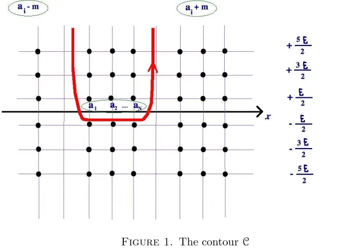
and the contour Cthat goes around the points al+kε, k ≥0. It can be deformed to

go along the real line, when al∈R+₂ε, and Imε >0.

In the perturbative limit the Bethe equation derived from the superpotential (6.5) assumes the form:

(6.6)

Λ

ε

2N ai

ε

=Y

j6=i

−

Γ1 +ai−aj

ε

Γ1−ai−aj

ε

Figure 1. The contourC

which has the form of the ordinary Bethe ansatz equations for a system of interacting particles (x1, . . . , xN) with the factorizableS-matrix, which coincides with that of the

open Toda chain. The two-body S-matrix is that of the Liouville quantum mechanics.

6.2.2. The elliptic Calogero-Moser system. Let P(x) =QN

l=1(x−al), and

(6.7) Q(x) = P(x−m)P(x+m+ε)

P(x)P(x+ε) ,

G(x) = d

dxlog

(x+m+ε)(x−m)(x−ε) (x−m−ε)(x+m)(x+ε) Then: W(a, ε; q) =Wpert+Winst,

(6.8) Wpert = 1 2ετ

N

X

n=1

a2_n+

N

X

l,n=1

(̟ε(al−an)−̟ε(al−an−m−ε))

and Winst is given by (6.2) with the contour C in the complex plane that comes from infinity, goes around the points al+kε, l= 1, . . . , N,k= 0,1,2, . . ., and goes back to

infinity. It separates these points and the points al+lm+kε,l ∈Z, k=−1,−2, . . ..

The perturbative Bethe equations have the form similar to (6.6):

(6.9) qaiε =

Y

j6=i

Γai−aj

ε

Γai−aj

ε

Γ−m−ai+aj

ε

Γ−m+ai−aj

ε

6.2.3. Ruijsenaars-Schneider model. Let us denote: q=e−βε_{, t=e}−βm_{, z=e}−βx_{, w} l= eβal_{. The perturbative contribution is:}

Wpert = πiτ 2ε

N

X

n=1

a2_n+

N

X

l,n=1

(Πq(wl/wn)−Πq(twl/wn))

where

Πq(w) = 1 β

∞ X

n=1

wn n2_(1−qn₎ ∼

X

n∈Z

̟ε

log(w) + 2πin β

The P, Q, G functions are given by:

(6.10) P(x) =

N

Y

l=1

(1−wlz), Q(x) =

P(zt−1)P(qtz)

P(z)P(qz)

G(x) =z d dzlog

z2_{(z−tq)(1−tz)(1−qz)} (z−t)(z−q)(1−qtz)

We assume |q|,|t|,|wl|<1, and the contour Cis the unit circle |z|= 1.

6.2.4. The spectrum of observables. The spectrum of the type A quantum system is given by the solutions of the equations (2.17) with W(a, ε) given by (6.1). Let us denote the extremum of the functional (6.1) by ρA(x), ϕA(x). The spectrum of the

type B quantum system is given by the solutions of the ”dual” equations

(6.11) ai=εni, ni∈Z

With these ai’s one can again define the functional (6.1) and study its extremum ρB(x), ϕB(x).

The eigenvalues of the quantized Hamiltonians

Hk=

Z

dzd¯ztrΦ(z)k =

N

X

l=1

pk_l +. . .:

are given respectively, for the type A and type B models:

(6.12) E_k=

N

X

l=1

ak_l +k

Z

C

dx(x+ε)k−1−xk−1ρA,B(x),

In particular:

(6.13) E₂ =εq d

6.2.5. On the relation between the type A and the type B models. The N = 2∗ _gauge

theory becomes the N = 4 super-Yang-Mills theory in the ultraviolet. The latter has the celebrated Montonen-Olive SL2(Z) symmetry. In particular, the S-duality transformation maps the gauge theory with the gauge group G and the coupling τ to the gauge theory with the gauge group L_{Gand the coupling−}1

hτ, for some integerh=

1,2,3. When the theory is perturbed by the mass term, the S-duality symmetry still acts. We claim it maps the type A model of the elliptic Calogero-Moser system with the modular parameterτ to the type B model with the modular parameter−1_τ. The special coordinates ai map to τ ai. The modularity of the effective twisted superpotential is

clearly supported by the expansion (6.17).

6.2.6. More details and the origin of integral equation. Here we give more details in regard to the origin of claims from previous sub-sections. We do it for the case of the

N= 2∗ _{theory (the relativistic case is studied analogously, along the lines of [47, 48]).}

One starts with the contour integral representation [1, 8, 7, 6] for the instanton partition function in the general Ω-background:

(6.14) Zinst(a; q, m, ε1, ε2) =

∞ X

k=0 qk

k!

Z

Rk

Y

1≤I<J≤k

D(φIJ) k

Y

I=1

Q(φI)

ε(m+ε1)(m+ε2)

ε1ε2m(m+ε) dφI

2πi,

where φIJ =φI−φJ,

D(x) = x

2_(x2_−ε2_)(x2_−(m+ε

1)2)(x2−(m+ε2)2) (x2_−ε2

1)(x2−ε22)(x2−m2)(x2−(m+ε)2)

,

and Q(x) was introduced in (6.7). Next use the observation, reported earlier in [49, 18], that (6.14) is a partition function of a one-dimensional non-ideal gas of particles

φ1, . . . , φk subject to the external potential

(6.15) Uext(x) =−log

Q(x)(m+ε1)(m+ε2)ε

ε1ε2m(m+ε)

and a pair-wise interaction potential

(6.16) Vint(x) =−log (D(x))

The free energy of this gaz can be analyzed using Mayer expansion [51, 52, 53]. The subtlety with the ε2 → 0 limit is the clustering of the instanton particles, which leads to the multiple vertices of a given valency, labelled by an arbitrary positive integer k

(the number of instantons in a given cluster) weighted by the partition function of a simpler one-dimensional gas

1

k!εk₂

Z

Rk

δ X

I φI

!

dkφ Y

1≤I<J≤k φIJ φIJ +ε2

to (6.2), (6.3) with the propagator function G(x) given by:

G(x) = Limitε2→0

D(x)−1

ε2

6.3. The sum over partitions. The U(N) instanton partition function can also be written as a sum over N-tuples of partitions λ(1)_{, . . . , λ}(N)_{, which represent various} configurations of instantons sitting on top of each other in R4. This representation can be effectively used to compute the first few terms in the q-expansion of Winst, or the first terms in the _a12 expansion, say, in the region |ai−aj| ≫ |ε|:

Winst(a, ε;m,q) = N m(m+ε)

ε ϕ(q) +

(6.17) +1

ε

X

i6=j

m2(m+ε)2 (ai−aj)2−ε2 q

dϕ(q)

dq +. . . where

(6.18) ϕ(q) = log

∞ Y

7. Discussion

To conclude we briefly review the relation of our results to some recent work. The periodic Toda system: In [19] the wavefunctions of the periodic Toda chain are constructed in the form of integrals involving the solution Q(x) of the Baxter equation. In order for the wavefunction to belong to the L2 _{Hilbert space the zeroes}

δ1, . . . , δN of Q must obey the quantization condition (in [19] the solution of Baxter equation is divided by the periodic function QN

i=1sinh

x−δi

ε

). We claim that the

quantization conditionsof [19] are equivalent to our Bethe equations for the pureN= 2

U(N) gauge theory, with the identification δi = ai. We have therefore provided the

YY function for the quantization conditons in the periodic Toda chain. Note that our perturbative equation (6.6) is derived for the periodic Toda system in [56] from the approximate analysis of the Baxter equation. The observation of [56] was very helpful in relating our two dimensional story [4, 5] to the four dimensional one.

In [57] aquasimappartial compactification of the moduli space of holomorphic maps of a sphere into the affine flag variety LG/T is studied, and the corresponding J -function [28] is shown to obey tautologically a non-stationary version of the periodic Toda equation, the affine analogue of the result [29] for the G/T type A sigma model. The intersection homology methods of [57] are not applicable, it seems, to other quan-tum integrable systems. The questions addressed in the current paper do not appear in [57], while the interesting setup of [57] has its own place (4.10) in our general story, having to do with the four dimensional gauge theory in the presence of defects [50], which we discuss elsewhere [13].

The elliptic Calogero-Moser system: In [20] the quantum N-particle elliptic Calogero-Moser system for theAN−1 system, for the integer coupling parameter ν was studied using the critical level limit of the free field representation of the conformal blocks of the WZW conformal field theory on a torus. The wavefunctions in [20] are written in terms of

m= N(N −1)

2 (ν−1)

parameters t(αii), αi = 1, . . . , i(ν−1), i= 1, . . . , N −1, obeying the elliptic Bethe-like equations, which are derived from the Yang-Yang function

Y(t(_αi);ξ1, . . . , ξN) = 2πi N

X

i=1





1 2τ ξ

2

i +ξi i(ν−1)

X

α=1

t(_αi)



−S(t(_αi);τ)

with the quasimomentaξ1, . . . , ξN being the fixed parameters. One can supplement the

Bethe equations of [20] by thequantization conditionsξ1 =ϑ+n1, ξ2 =ϑ+n2, . . . , ξN = ϑ+nN, withni ∈Z. We conjecture

(7.1) Crit_t(i)

α ,Pi(ν_α=1−1)t(i)α =aiS(t (i)

α ;τ) = ˜Weff(a1, . . . , aN;−νε, ε, τ)

on the elliptic curve Eτ. The equivalence (7.1) suggests an interesting duality between

the N = 2∗ _{theory in the special Ω background with the coupling τ and the quiver}

gauge theory.

In [54] a partial resummation of the quantum mechanical perturbation theory around the trigonometric Sutherland model is proposed, leading to an equation on the eigen-value of the ˆH2 operator of the elliptic Calogero-Moser system, for an arbitrary value of the coupling ν. The relation of this approach to the YY-function formalism is not clear to us at the moment.

Parallel developments: There are several recent developments which we feel are related to our story, including the obvious ones, such as the integrability in the AdS/CFT context, but also [43, 55, 58, 59, 60, 61]. It is tempting to conclude from the convergence of these topics that the planarN= 4 super-Yang-Mills is equivalent to the union of the vacuum sectors of all gauge theories with eight supercharges (N = 2 in four dimensions).

We would like to return to all these questions in the future.

References

[1] G. Moore, N. Nekrasov, S. Shatashvili, Integration over the Higgs branches, Comm. Math. Phys. 209 (2000) 97-121, arXiv:hep-th/9712241.

[2] A. Gerasimov, S. Shatashvili,Higgs Bundles, Gauge Theories and Quantum Groups,Comm. Math. Phys. 277 (2008) 323-367, arXiv:hep-th/0609024.

[3] A. Gerasimov, S. Shatashvili,Two-dimensional Gauge Theories and Quantum Integrable Systems, In “From Hodge Theory to Integrability and TQFT: tt*-geometry”, pp. 239-262, R. Donagi and K. Wendland, Eds., Proc. of Symposia in Pure Mathematics Vol. 78, American Mathematical Society, Providence, Rhode Island, 2008; arXiv:0711.1472.

[4] N. Nekrasov, S. Shatashvili, Supersymmetric vacua and Bethe ansatz, In “Cargese 2008, Theory and Particle Physics: the LHC perspective and beyond”, arXiv:0901.4744.

[5] N. Nekrasov, S. Shatashvili,Quantum integrability and supersymmetric vacua,Prog. Theor. Phys. Suppl. 177:105-119, 2009, arXiv:0901.4748.

[6] N. Nekrasov,Seiberg-Witten prepotential from instanton counting,Adv. Theor. Math. Phys. 7:831-864, 2004, hep-th/0206161.

[7] A. Losev, N. Nekrasov, S. Shatashvili,Testing Seiberg-Witten solution,In “Cargese 1997, Strings, branes and dualities” 359-372, hep-th/9801061.

[8] G. Moore, N. Nekrasov, S. Shatashvili,D particle bound states and generalized instantons,Commun. Math. Phys. 209 (2000) 77-95, hep-th/9803265.

[9] N. Seiberg, E. Witten,Monopole Condensation, And Confinement InN= 2Supersymmetric Yang-Mills Theory, arXiv:hep-th/9407087, Nucl. Phys. B426 (1994) 19-52; Erratum-ibid.B430:485-486, 1994

[10] A. Gorsky, I. Krichever, A. Marshakov, A. Mironov, A. Morozov,Integrability and Seiberg-Witten exact solution,Phys. Lett. B355:466-474,1995, hep-th/9505035.

[11] R. Donagi, E. Witten, Supersymmetric Yang-Mills theory and integrable systems, Nucl. Phys. B460:299-334, 1996, hep-th/9510101.

[12] C. N. Yang, C. P. Yang, Thermodinamics of a one-dimensional system of bosons with repulsive delta-function interaction,J. Math. Phys. 10 (1969), 1115.

[13] N. Nekrasov, S. Shatashvili,Supersymmetric vacua and quantum integrability, to appear. [14] K. Hori, S. Katz, A. Klemm, R. Pandharipande, R. Thomas, C. Vafa, R. Vakil, E. Zaslow (Eds.),

Mirror symmetry, American Mathematical Society, Providence, 2003, 929p.

[16] H. Bethe,On the theory of metals. 1. Eigenvalues and eigenfunctions for the linear atomic chain, Z. Phys. 71: 205-226, 1931.

[17] A. Losev, A. Marshakov, N. Nekrasov,Small instantons, little strings and free fermions,In “Shif-man, M. (ed.) et al.: From fields to strings, vol. 1”, 581-621, hep-th/0302191.

[18] A. Marshakov, N. Nekrasov, Extended Seiberg-Witten Theory and Integrable Hierarchy, JHEP 0701:104, 2007, hep-th/0612019.

[19] S. Kharchev, D. Lebedev, Integral representations for the eigenfunctions of quantum open and periodic Toda chains from QISM formalism, arXiv:hep-th/0007040, J. Phys. A34 (2001) 2247-2258 [20] G. Felder, A. Varchenko, Integral representation of solutions of the elliptic Knizhnik– Zamolodchikov–Bernard equations, arXiv:hep-th/9502165, Int. Math. Res. Notices (1995) 221-233. [21] H. Braden, I. Krichever, eds. The Seiberg-Witten and Whitham Equations, Gordon and Breach

Science Publishers, 2000.

[22] N. Nekrasov, A. Okounkov,Seiberg-Witten theory and random partitions, hep-th/0306238. [23] Al. Zamolodchikov,Thermodynamic Bethe Ansatz in Relativistic Models. Scaling 3-state Potts and

Lee-Yang Models, Nucl. Phys. B342 (1990) 695.

[24] C. Destri, H. J. de Vega,New approach to thermal Bethe Ansatz, Phys. Rev. Lett. 69 (1992) 2313. [25] V. Bazhanov, S. Lukyanov and A. Zamolodchikov, Integrable quantum field theories in finite

vol-ume: excited state energies, Nucl. Phys. B489 (1997) 487-531, hep-th/9607099.

[26] P. Dorey and R. Tateo, Excited states by analytic continuation of TBA equations, Nucl. Phys. B482 (1996) 639-659, hep-th/9607167.

[27] J. Teschner,On the spectrum of the sinh-Gordon model in finite volume, hep-th/0702214. [28] A. Givental,Equivariant Gromov-Witten Invariants, arXiv:alg-geom/9603021

[29] A. Givental,Stationary Phase Integrals, Quantum Toda Lattices, Flag Manifolds and the Mirror Conjecture, arXiv:alg-geom/9612001

[30] L. Faddeev, E. Sklyanin, L. Takhtajan, Quantum inverse problem method, Theor. Math. Phys. 40:2 (1980) 688-706, Teor. Mat. Fiz. 40:194-220,1979 (in Russian)

[31] L. Takhtajan, L. Faddeev, The Quantum method of the inverse problem and the Heisenberg XYZ model,Published in Russ. Math. Surveys 34:11-68,1979, Usp. Mat. Nauk 34:13-63, 1979.

[32] L. Faddeev,How algebraic Bethe ansatz works for integrable model, hepth/9605187

[33] E. Sklyanin, Separation of variables - new trends, Prog. Theor. Phys. Suppl. 118 (1995) 35-60, e-Print: solv-int/9504001

[34] R. Baxter,Exactly solved models in statistical mechanics, Academic Press, London 1982

[35] F. A. Smirnov, Structure of Matrix Elements in Quantum Toda Chain, J. Phys. A. 31 (1998) 8953,arXiv:math-ph/9805011

[36] A. Beilinson, V. Drinfeld, Quantization of Hitchin’s integrable system and Hecke eigensheaves, preprint (ca. 1995), http://www.math.uchicago.edu arinkin/langlands/

[37] I. Krichever, Elliptic solutions of the KadomtsevPetviashvili equation and integrable systems of particles, Funkts. Anal. Prilozh., 14:4 (1980), 4554

[38] V. Inozemtsev,The Finite Toda Lattices, Comm. Math. Phys.121 (1989) 629-638

[39] G. Lam´e,Sur les surfaces isothermes dans les corps homognes en quilibre de temprature, J. Math. Pures Appl. 2 (1837), 147188.

[40] N. Nekrasov, Holomorphic bundles and many-body systems, Commun. Math. Phys. 180 (1996) 587-604, hep-th/9503157.

[41] A. Gorsky, N. Nekrasov,Elliptic Calogero-Moser System from Two Dimensional Current Algebra, hep-th/9401021.

[42] D. Gaiotto, N= 2 dualities, arXiv:0904.2715v1

[43] A. Kapustin, E. Witten, Electric-Magnetic Duality And The Geometric Langlands Program, arXiv:hep-th/0604151

[44] S. Ruijsenaars, H. Schneider,A new class of integrable systems and its relation to solitons, Ann. Phys. (NY) 170 (1986) 370–405.

[45] S. Ruijsenaars, Complete integrability of relativistic Calogero-Moser systems and elliptic function identities, Comm. Math. Phys. 110 (1987) 191–213.

[47] N. Nekrasov, Five dimensional gauge theories and the relativistic gauge theories, arXiv:hep-th/9609219, Nucl.Phys.B_{531 (1998) 323-344}

[48] N. Nekrasov, S. Shadchin, ABCD of instantons, Comm. Math. Phys. 252 (2004) 359-391 , arXiv:hep-th/0404225

[49] N. Nekrasov,Random partitions, topological strings and Mayer expansion,lectures at the Univer-sity of Amsterdam conference “On random Partitions and Topological Strings”, June 2005. [50] N. Nekrasov, Gauge theory special functions: Z_{-functions for instantons with defects, lecture at}

the DARPA meeting,Langlands program and gauge theory, IAS, Princeton, March 2004 [51] J. Mayer, M. G. Mayer,Statistical Mechanics, New York 1940

[52] J. Mayer, E. Montroll,Molecular distributions, J. Chem. Phys.9_{(1941) 2-16}

[53] A. Polyakov,Microscopic description of critical phenomena JETP 55 (1968) 1026-1038

[54] E. Langmann, An explicit solution of the (quantum) elliptic Calogero-Sutherland model, arXiv:math-ph/0407050

[55] S. Gukov, E. Witten,Branes and Quantization, arXiv:0809.0305

[56] C. Ahn, V. Fateev, C. Kim, C. Rim, B. Yang, Reflection Amplitudes of ADE Toda Theories and Thermodynamic Bethe Ansatz, arXiv:hep-th/9907072, Nucl.Phys. B565 (2000) 611-628

[57] A. Braverman,Instanton counting using affine Lie algebras I: equivariant J_{-functions of (affine)}

flag varieties and Whittaker vectors, arXiv:math/0401409

[58] M. Kontsevich, Y. Soibelman,Stability structures, motivic Donaldson-Thomas invariants and clus-ter transformations, arXiv:0811.2435

[59] L. Alday, J. Maldacena,Null polygonal Wilson loops and minimal surfaces in Anti-de-Sitter space, arXiv:0904.0663

[60] D. Gaiotto, G. Moore, A. Neitzke,Wall-crossing, Hitchin Systems, and the WKB Approximation, arXiv:0907.3987

[61] L. Alday, D. Gaiotto, Y. Tachikawa,Liouville Correlation Functions from Four-dimensional Gauge Theories, arXiv:0906.3219

IHES, Le Bois-Marie, 35 route de Chartres, Bures-sur-Yvette, 91440, France, Simons Center for Geometry and Physics, Stony Brook University, NY 11794 USA, E-mail: [email protected]