Mental Illness Detection at the World Well Being Project for the CLPsych 2015 Shared Task

Proceedings of the 2nd Workshop on Computational Linguistics and Clinical Psychology: From Linguistic Signal to Clinical Reality, pages 40–45,

Mental Illness Detection at the World Well-Being Project for the

CLPsych 2015 Shared Task

Daniel Preot¸iuc-Pietro1,2_{Maarten Sap}1_{H. Andrew Schwartz}1,2_{and Lyle Ungar}1,2 1_{Department of Psychology, University of Pennsylvania}

2_{Computer & Information Science, University of Pennsylvania}

[email protected]

Abstract

This article is a system description and report on the submission of the World Well-Being Project from the University of Pennsylvania in the ‘CLPsych 2015’ shared task. The goal of the shared task was to automatically determine Twitter users who self-reported having one of two mental illnesses: post traumatic stress dis-order (PTSD) and depression. Our system em-ploys user metadata and textual features de-rived from Twitter posts. To reduce the fea-ture space and avoid data sparsity, we con-sider several word clustering approaches. We explore the use of linear classifiers based on different feature sets as well as a combination use a linear ensemble. This method is agnos-tic of illness specific features, such as lists of medicines, thus making it readily applicable in other scenarios. Our approach ranked second in all tasks on average precision and showed best results at.1false positive rates.

1 Introduction

Mental illnesses are widespread globally ( ¨Ust¨un et al., 2004); for instance, 18.6% of US adults were suffering from a mental illness in 2012 (Abuse and Administration, 2012). Depression and post trau-matic stress disorder (PTSD) are some of the most common disorders, reaching up to 6.6% and 3.5% prevalence respectively in a 12 month period in the US (Kessler et al., 2003; Kessler et al., 2005). How-ever, these are often argued to be under-estimates of the true prevalence (Prince et al., 2007). This is in part because those suffering from depression and PTSD do not typically seek help for their symptoms and partially due to imperfect screening methods

currently employed. Social media offers us an alter-native window into an individual’s psyche, allowing us to investigate how changes in posting behaviour may reflect changes in mental state.

The CLPsych 2015 shared task is the first evalua-tion to address the problem of automatically identi-fying users with diagnosis of mental illnesses, here PTSD or depression. The competition uses a corpus of users who self-disclosed their mental illness diag-noses on Twitter, a method first introduced in (Cop-persmith et al., 2014). The shared task aims to dis-tinguish between: (a) control users and users with depression, (b) control users and users with PTSD and (c) users with depression and users with PTSD. For our participation in this shared task, we treat the task as binary classification using standard reg-ularised linear classifiers (i.e. Logistic Regression and Linear Support Vector Machines). We use a wide range of automatically derived word clusters to obtain different representations of the topics men-tioned by users. We assume the information cap-tured by these clusters is complimentary (e.g. se-mantic vs. syntactic, local context vs. broader con-text) and combine them using a linear ensemble to reduce classifier variance and improve accuracy. Our classifier returns for each binary task a score for each user. This enables us to create a ranked list of use in our analysis.

The results are measured on average precision, as we are interested in evaluating the entire ranking. On the official testing data, our best models achieve over

.80average precision (AP) for all three binary tasks, with the best model reaching .869 AP on predict-ing PTSD from controls in the official evaluation. A complementary qualitative analysis is presented in (Preot¸iuc-Pietro et al., 2015).

2 System Overview

In our approach, we aggregate the word counts in all of a user’s posts, irrespective of their timestamp and the word order within (a bag-of-words approach). Each user in the dataset is thus represented by a dis-tribution over words. In addition, we used automat-ically derived groups of related words (or ‘topics’) to obtain a lower dimensional distribution for each user. These topics, built using automatic clustering methods from separate large datasets, capture a set of semantic and syntactic relationships (e.g. words reflecting boredom, pronouns). In addition, we use metadata from the Twitter profile of the user, such as number of followers or number of tweets posted. A detailed list is presented in the next section. We trained three standard machine learning binary clas-sifiers using these user features and known labels for Controls, Depressed and PTSD users.

Data

The data used for training consisted of 1,145 Twit-ter users, labeled as Controls, Depressed and PTSD. This dataset was provided by the shared task organ-isers (Coppersmith et al., 2015). From training and testing we removed 2 users as they had posted less than 500 words and thus their feature vectors were very sparse and uninformative. Dataset statistics are presented in Table 1. Age and gender were provided by the task organisers and were automatically de-rived by the method from (Sap et al., 2014).

Control Depressed PTSD Number of users 572 327 246

Avg. age 24.4 21.7 27.9

% female 74.3% 69.9% 67.5% Avg. # followers 1,733 1,448 1,784 Avg. # friends 620 836 1,148 Avg. # times listed 22 17 29

Avg. # favourites 1,195 3,271 5,297 Avg. # statuses 10,772 17,762 16,735 Avg. # unigrams 31,083 32,938 38,337

Table 1: Descriptive statistics for each of the three categories of users.

3 Features and Methods 3.1 Features

We briefly summarise the features used in our pre-diction task. We divide them into user features and textual features.

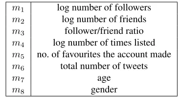
Metadata Features (Metadata) The metadata features are derived from the user information avail-able from each tweet that were not anonymised by the organizers. Table 2 introduces the eight features in this category.

m1 log number of followers

m2 log number of friends

m3 follower/friend ratio

m4 log number of times listed

m5 no. of favourites the account made

m6 total number of tweets

m7 age

m8 gender

Table 2: Metadata features for a Twitter user.

Unigram Features (Unigram) We use unigrams as features in order to capture a broad range of textual information. First, we tokenised the Twitter posts into unigrams using our tailored version1 _of

Chris Potts’ emoticon-aware HappyFunTokenizer. We use the unigrams mentioned by at least 1% of users in the training set, resulting in a total of 41,687 features.

Brown Clusters (Brown) Using all unigrams may cause different problems in classification. The feature set in this case is an order of mag-nitude larger than the number of samples (∼

40,000 ∼1000), which leads to sparse features and may cause overfitting. To alleviate this prob-lem, we use as features different sets of words which are semantically or syntactically related i.e. ‘topics’. These are computed on large corpora unrelated to our dataset in order to confer generality to our meth-ods.

The first method is based on Brown cluster-ing (Brown et al., 1992). Brown clustercluster-ing is a HMM-based algorithm that partitions words hierar-chically into clusters, building on the intuition that

the probability of a word’s occurrence is based on the cluster of word directly preceding it. We use the clusters introduced by Owoputi et al. (2013) which use the method of Liang (2005) to cluster 216,856 tokens into a base set of 1000 clusters using a dataset of 56 million English tweets evenly distributed from 9/10/2008 to 8/14/2012.

NPMI Word Clusters (NPMI) Another set of clusters is determined using the method presented in (Lampos et al., 2014). This uses a word to word similarity matrix computed over a large ref-erence corpus of 400 million tweets collected from 1/2/2011 to 2/28/2011. The word similarity is mea-sured using Normalised Pointwise Mutual Infor-mation (NPMI). This inforInfor-mation-theoretic measure indicates which words co-occur in the same con-text (Bouma, 2009) where the concon-text is the entire tweet. To obtain hard clusters of words we use spec-tral clustering (Shi and Malik, 2000; Ng et al., 2002). This methods was shown to deal well with high-dimensional and non-convex data (von Luxburg, 2007). In our experiments we used 1000 clusters from 54,592 tokens.

Word2Vec Word Clusters (W2V) Neural meth-ods have recently been gaining popularity in or-der to obtain low-rank word embeddings and ob-tained state-of-the-art results for a number of seman-tic tasks (Mikolov et al., 2013b).

These methods, like many recent word embed-dings, also allow to capture local context order rather than just ‘bag-of-words’ relatedness, which leads to also capture syntactic information. We use the skip-gram model with negative sampling (Mikolov et al., 2013a) to learn word embeddings from a cor-pus of 400 million tweets also used in (Lampos et al., 2014). We use a hidden layer size of 50 with the Gensim implementation.2_{We then apply spectral}

clustering on these embeddings to obtain hard clus-ters of words. We create 2000 clusclus-ters from 46,245 tokens.

GloVe Word Clusters (GloVe) A different type of word embeddings was introduced by (Penning-ton et al., 2014). This is uses matrix factorisation on a word-context matrix which preserves word or-der and claims to significantly outperform previous

2_{https://radimrehurek.com/gensim/}

neural embeddings on semantic tasks. We use the pre-trained Twitter model from the author’s website3

built from 2 billion tweets. In addition to the largest layer size (200), we also use spectral clustering as explained above to create 2000 word clusters from 38,773 tokens.

LDA Word Clusters (LDA) A different type of clustering is obtained by using topic models, most popular of which is Latent Dirichlet Allocation (Blei et al., 2003). LDA models each post as being a mixture of different topics, each topic representing a distribution over words, thus obtaining soft clus-ters of words. We use the 2000 clusclus-ters introduced in (Schwartz et al., 2013), which were computed over a large dataset of posts from 70,000 Facebook users. These soft clusters should have a slight dis-advantage in that they were obtained from Facebook data, rather than Twitter as all previously mentioned clusters and our dataset.

LDA ER Word Clusters (ER) We also use a dif-ferent set of 500 topics. These were obtained by per-forming LDA on a dataset of∼700Facebook user’s posts who reported to the emergency room and opted in a research study.

3.2 Methods

We build binary classifiers to separate users being controls, depressed or having PTSD. As classifiers, we use linear methods as non-linear methods haven’t shown improvements over linear methods in our pre-liminary experiments. We use both logistic regres-sion (LR) (Freedman, 2009) with Elastic Net regu-larisation (Zou and Hastie, 2005) and Support Vec-tor Machines (LinSVM) with a linear kernel (Vap-nik, 1998). We used the implementations of both classifiers from ScikitLearn (Pedregosa et al., 2011) which use Stochastic Gradient Descent for infer-ence.

A vital role for good performance in both classi-fiers is parameter tuning. We measure mean average precision on our training set using 10 cross-fold val-idation and 10 random restarts and optimise param-eters using grid search for each feature set individu-ally.

Different feature sets are expected to contribute

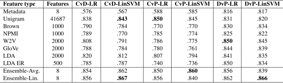
Feature type Features CvD-LR CvD-LinSVM CvP-LR CvP-LinSVM DvP-LR DvP-LinSVM

Metadata 8 .576 .567 .588 .585 .816 .817

Unigram 41687 .838 .843 .850 .845 .831 .820

Brown 1000 .790 .784 .770 .770 .830 .834

NPMI 1000 .789 .770 .785 .774 .825 .822

W2V 2000 .808 .791 .786 .775 .850 .845

GloVe 2000 .788 .784 .780 .761 .844 .839

LDA 2000 .820 .812 .807 .794 .841 .835

LDA ER 500 .785 .787 .740 .736 .850 .834

Ensemble-Avg. 8 .854 .862 .850 .860 .856 .839

Ensemble-Lin. 8 .856 .867 .856 .840 .862 .866

Table 3: Average precision for each individual set of features and both classifiers. The three binary classifi-cation tasks are Controls vs. Depressed (CvD), Controls vs. PTSD (CvP) and Depressed vs. PTSD (DvP).

to the general classification results with different in-sights. A combination of features is thus preferable in order to boost performance and also reduce vari-ance or increase robustness.

We create an ensemble of classifiers, each of which uses the different textual feature sets de-scribed in the previous section. The predicted scores for each model are used to train a logistic regression classifier in order to identify the weights assigned to each classifier before their output is combined (Ensemble-Lin.). We also experimented with a non-weighted combination of classifiers ( Ensemble-Avg.).

4 Results

The results of our methods on cross-validation are presented in Table 3. Results using different feature sets show similar values, with all unigram features showing overall best results. However, we expect that each set of features will contribute with distinc-tive and complimentary information.

The ensemble methods show minor, but consis-tent improvement over the scores of each individual user set. The linear combination of different classi-fiers shows better performance compared to the av-erage by appropriately down-weighting less infor-mative sets of features.

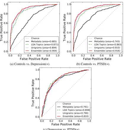
Figure 1 shows the three ROC (Receiver Operator Characteristic) curves for our binary classification tasks. These curves are specifically useful for med-ical practitioners as the classification threshold can be adjusted to obtain an application specific level of false positives.

For example, we highlight that at a false positive rate of0.1, we reach a true positive rate of 0.8 for separating Controls from users with PTSD and of

0.75 for separating Controls from depressed users. Distinguishing PTSD from depressed users is harder at small false positive rates, with only ∼ 0.4 true positive rate.

5 Discussion and Conclusions

This paper reported on the participation of the World Well-Being Project in the CLPsych 2015 shared task on identifying users having PTSD or depression.

Our methods were based on combining linear classifiers each using different types of word clus-ters. The methods we presented were designed to be as task agnostic as possible, aiming not to use medi-cal condition specific keywords or data. We thus ex-pect similar methods to perform well in identifying other illnesses or conditions.

This generalised approach yielded results ranking second in the shared task, scoring above0.80on all tasks and reaching up to0.87for one of the binary tasks. Further analysis shows that our models per-form especially well at small false positive rates (up to 0.8 true positive rate at 0.1 false positive rate) where it ranked first.

0.0

0.2

0.4

0.6

0.8

1.0

False Positive Rate

0.0

0.2

0.4

0.6

0.8

1.0

True Positive Rate

LDA Topics (area=0.871) Unigrams (area=0.894) Ensemble (area=0.904)

(a) Controls vs. Depression(+).

0.0

0.2

0.4

0.6

0.8

1.0

False Positive Rate

0.0

0.2

0.4

0.6

0.8

1.0

True Positive Rate

LDA Topics (area=0.883) Unigrams (area=0.910) Ensemble (area=0.916)

(b) Controls vs. PTSD(+).

0.0

0.2

0.4

0.6

0.8

1.0

False Positive Rate

0.0

0.2

0.4

0.6

0.8

1.0

True Positive Rate

LDA Topics (area=0.808) Unigrams (area=0.790) Ensemble (area=0.810)

(c) Depression vs. PTSD(+).

Figure 1: ROC curves and area under the curve for a selected set of features using Linear Support Vector Classification. (+) denotes positive class.

References

Substance Abuse and Mental Health Services Adminis-tration. 2012. Results from the 2010 National Sur-vey on Drug use and Health: Mental Health Findings.

NSDUH series H-42, HHS publication no.(SMA) 11-4667.

David M. Blei, Andrew Y. Ng, and Michael I. Jordan. 2003. Latent Dirichlet Allocation. Journal of Ma-chine Learning Research, 3:993–1022.

Gerlof Bouma. 2009. Normalized (pointwise) Mu-tual Information in collocation extraction. InBiennial GSCL Conference, pages 31–40.

Peter F. Brown, Peter V. deSouza, Robert L. Mercer, Vin-cent J. Della Pietra, and Jenifer C. Lai. 1992. Class-based N-gram Models of Natural Language. Compu-tational Linguistics, 18(4):467–479.

Glen Coppersmith, Mark Dredze, and Craig Harman. 2014. Quantifying Mental Health Signals in Twitter. In52nd Annual Meeting of the Association for Com-putational Linguistics, ACL.

Glen Coppersmith, Mark Dredze, Craig Harman, Kristy Hollingshead, and Margaret Mitchell. 2015. CLPsych 2015 shared task: Depression and PTSD on Twitter. In

Lin-guistics and Clinical Psychology: From Linguistic Sig-nal to Clinical Reality, NAACL.

David Freedman. 2009. Statistical models: theory and practice. Cambridge University Press.

Ronald C Kessler, Patricia Berglund, Olga Demler, Robert Jin, Doreen Koretz, Kathleen R Merikangas, A John Rush, Ellen E Walters, and Philip S Wang. 2003. The epidemiology of major depressive disorder: results from the National Comorbidity Survey Replica-tion (NCS-R). Journal of the American Medical Asso-ciation, 289(23):3095–3105.

Ronald C Kessler, Wai Tat Chiu, Olga Demler, and Ellen E Walters. 2005. Prevalence, severity, and co-morbidity of 12-month dsm-iv disorders in the national comorbidity survey replication. Archives of general psychiatry, 62(6):617–627.

Vasileios Lampos, Nikolaos Aletras, Daniel Preot¸iuc-Pietro, and Trevor Cohn. 2014. Predicting and char-acterising user impact on Twitter. InProceedings of the 14th Conference of the European Chapter of the Association for Computational Linguistics, EACL. Percy Liang. 2005. Semi-supervised Learning for

Natu-ral Language. InMaster’s Thesis, MIT.

Tomas Mikolov, Kai Chen, Greg Corrado, and Jeffrey Dean. 2013a. Efficient estimation of word representa-tions in vector space. InProceedings of Workshop at the International Conference on Learning Representa-tions, ICLR.

Tomas Mikolov, Wen tau Yih, and Geoffrey Zweig. 2013b. Linguistic Regularities in Continuous Space Word Representations. InProceedings of the 2010 an-nual Conference of the North American Chapter of the Association for Computational Linguistics, NAACL, pages 746–751.

Andrew Y. Ng, Michael I. Jordan, and Yair Weiss. 2002. On Spectral Clustering: Analysis and an algorithm. In

Advances in Neural Information Processing Systems, NIPS, pages 849–856.

Olutobi Owoputi, Brendan O’Connor, Chris Dyer, Kevin Gimpel, Nathan Schneider, and A. Noah Smith. 2013. Improved Part-of-Speech Tagging for Online Conver-sational Text with Word Clusters. InProceedings of the 2013 Conference of the North American Chapter of the Association for Computational Linguistics: Hu-man Language Technologies, NAACL.

Fabian Pedregosa, Gael Varoquaux, Alexandre Gram-fort, Vincent Michel, Bertrand Thirion, Olivier Grisel, Mathieu Blondel, Peter Prettenhofer, Ron Weiss, Vin-cent Dubourg, Jake Vanderplas, Alexandre Passos, David Cournapeau, Matthieu Brucher, Matthieu Per-rot, and Edouard Duchesnay. 2011. Scikit-learn: Ma-chine Learning in Python. Journal of Machine Learn-ing Research, 12:2825–2830.

Jeffrey Pennington, Richard Socher, and Christopher D. Manning. 2014. GloVe: Global Vectors for Word Rep-resentation. InProceedings of the 2014 Conference on Empirical Methods in Natural Language Processing, EMNLP.

Daniel Preot¸iuc-Pietro, Johannes Eichstaedt, Gregory Park, Maarten Sap, Laura Smith, Victoria Tobolsky, H. Andrew Schwartz, and Lyle Ungar. 2015. The Role of Personality, Age and Gender in Tweeting about Mental Illnesses. InProceedings of the Workshop on Computational Linguistics and Clinical Psychology: From Linguistic Signal to Clinical Reality, NAACL. Martin Prince, Vikram Patel, Shekhar Saxena, Mario

Maj, Joanna Maselko, Michael R Phillips, and Atif Rahman. 2007. No health without mental health. The Lancet, 370(9590):859–877.

Maarten Sap, Gregory Park, Johannes Eichstaedt, Mar-garet Kern, Lyle Ungar, and H Andrew Schwartz. 2014. Developing Age and Gender Predictive Lexica over Social Media. InProceedings of the 2014 Confer-ence on Empirical Methods in Natural Language Pro-cessing, EMNLP, pages 1146–1151.

H Andrew Schwartz, Johannes C Eichstaedt, Margaret L Kern, Lukasz Dziurzynski, Stephanie M Ramones, Megha Agrawal, Achal Shah, Michal Kosinski, David Stillwell, Martin EP Seligman, and Lyle H Ungar. 2013. Personality, Gender, and Age in the Language of Social Media: The Open-Vocabulary Approach.

PLoS ONE.

Jianbo Shi and Jitendra Malik. 2000. Normalized cuts and image segmentation. Transactions on Pattern Analysis and Machine Intelligence, 22(8):888–905. TB ¨Ust¨un, Joseph L Ayuso-Mateos, Somnath Chatterji,

Colin Mathers, and Christopher JL Murray. 2004. Global burden of depressive disorders in the year 2000.

The British journal of psychiatry, 184(5):386–392. Vladimir N Vapnik. 1998. Statistical learning theory.

Wiley, New York.

Ulrike von Luxburg. 2007. A tutorial on Spectral Clus-tering.Statistics and computing, 17(4):395–416. Hui Zou and Trevor Hastie. 2005. Regularization and