D S Sharma, R Sangal and A K Singh. Proc. of the 13th Intl. Conference on Natural Language Processing, pages 208–218, Varanasi, India. December 2016. c2016 NLP Association of India (NLPAI)
Learning Non-Linear Functions for Text Classification
Cohan Sujay Carlos Aiaioo Labs
Bangalore India
Geetanjali Rakshit IITB-Monash Research Academy
Mumbai India
Abstract
In this paper, we show that generative clas-sifiers are capable of learning non-linear decision boundaries and that non-linear generative models can outperform a num-ber of linear classifiers on some text cate-gorization tasks.
We first prove that 3-layer multinomial hierarchical generative (Bayesian) classi-fiers, under a particular independence as-sumption, can only learn the same lin-ear decision boundaries as a multinomial naive Bayes classifier.
We then go on to show that making a dif-ferent independence assumption results in nonlinearization, thereby enabling us to learn non-linear decision boundaries. We finally evaluate the performance of these non-linear classifiers on a series of text classification tasks.
1 Introduction
Probabilistic classifiers predict a class c given a
set offeaturesF of the data point being classified,
by selecting the most probable class given the fea-tures, as shown in Equation 1.
arg max
c P(c|F) (1)
Bayesian classifiers, also known as generative classifiers, are those that learn a model of the joint
probabilityP(F, c)of the inputsF and labelsc∈
C(Ng and Jordan, 2001), and use the Bayes rule
(2) to invert probabilities of the featuresF given
a classcinto a prediction of the classcgiven the
featuresF.
P(c|F) = P(F|c)×P(c)
P(F) (2)
2-layer classifiers such as the perceptron and the
naive Bayes classifier are only capable of learning linear decision boundaries (Minsky and Papert, 1988) passing through the origin (if learning a multinomial probability distribution), or quadratic decision boundaries (with a Gaussian probability distribution or kernel).
The multilayer perceptron, a 3-layer classifier
with an input layer, a hidden layer and an output layer, is capable of learning non-linear decision boundaries (Cybenko, 1989; Andoni et al, 2014). It is therefore only to be expected that3-layer
gen-erative models should also be capable of learning the same. However, it turns that under certain
conditions, 3-layer generative models for
classi-fication are only as powerful as 2-layer models,
and under other conditions, are capable of learn-ing non-linear decision boundaries.
In this paper, we study 3-layer hierarchical
multinomial generative models, and define the conditions under which their decision boundaries are linear or non-linear. The main contributions of the paper are the following:
• We prove that a certain set of independence
assumptions results in linear decision bound-aries and identical classification performance to a naive Bayes classifier.
• We demonstrate that a different set of
in-dependence assumptions makes models with the same parameters capable of learning linear decision boundaries and certain non-linear functions, for instance, a scaled and shifted XOR function.
• We show through experiments that such
non-linear hierarchical Bayesian models can outperform many commonly used machine learning models at certain text classification tasks.
2 Related Work
Deep learning is a term used to describe any method of machine learning involving the use of multiple processing layers to learn representations of data (LeCun et al., 2015; Bengio, 2009).
2.1 Neural Network Models
Two machine learning algorithms used in deep learning are the multilayer perceptron (Rumelhart et al, 1986) and the autoencoder (Alex et al, 2011), both of which are neural networks (Wang and Ye-ung, 2016).
2.2 Probabilistic Graphical Models
Probabilistic graphical models are concise graph-based representations of probability distributions over possibly complex and high-dimensional spaces, with the nodes representing variables of interest and various properties of the graph representing functions interpretable as probabili-ties (Koller and Friedman, 2009). Probabilistic graphical models are usually of one of two types, depending on whether their edges are directed or undirected.
Undirected probabilistic graphical models (also known as Markov random fields) have undirected edges and are models of probability distributions whose factorization is a function of the cliques in the graph (Wainwright and Jordan, 2008). They represent discriminative classifiers, which learn the probability of the labels given the features
P(c|F) directly (Ng and Jordan, 2001) without
first learningP(F|c)and then applying Bayesian
inversion. Two machine learning models used in deep learning - Boltzmann machines (Ack-ley et al, 1986) and restricted Boltzmann ma-chines (Smolensky, 1986) - are both undirected probabilistic graphical models (Fischer and Igel, 2012).
Directed probabilistic graphical models (also known as Bayesian networks) are on the other hand directed acyclic graphs where the factoriza-tion of the probability distribufactoriza-tion is a funcfactoriza-tion of the parent-child relationships in the graph.
2.3 Directed Probabilistic Graphical Models
For each vertex i ∈ 1. . . n in a directed
proba-bilistic graphical model and the set of ancestor ver-ticesa(i)ofi(vertices with a sequence of directed
edges leading to i), the random variables x1, x2
. . .xnattached to the nodes represent a family of
probabilistic distributions that factorise according to Equation 3.
P(x1, x2. . . xn) =
Y
1≤i≤n
P(xi|xa(i))
(3)
In this paper, we focus on a subset of directed probabilistic graphical models known as hierar-chical Bayesian models (Wainwright and Jordan, 2008).
2.4 Hierarchical Bayesian Models
Hierarchical Bayesian models are directed prob-abilistic graphical models in which the directed acyclic graph is a tree (each node that is not the root node has only one immediate parent). In these models the ancestorsa(i)of any nodeido not
con-tain any siblings (every pair of ancestors is also in an ancestor-descendent relationship). The fac-torization represented by a hierarchical Bayesian model is just a special case of Equation 3 (Wain-wright and Jordan, 2008). Such models naturally lend themselves to classification tasks because the root node can be used to represent the set of classes
Cand the leaf nodes the set of featuresF.
The naive Bayes classifier is a special case of a hierarchical Bayesian classifier because it consists of a tree that is only two layers deep (a root node and a layer of leaf nodes). So, for the naive Bayes classifier, Equation 3 reduces to Equation 4.
P(F, c) =P(F|c)P(c) = Y
f∈F
P(f|c)P(c) (4)
Naive Bayes classifiers are easy to train because all the nodes in the directed graph representation of a naive Bayes classifier are visible nodes. Since all the edge probabilities that need to be estimated in the learning step are between visible variables, they are easy to estimate.
With hierarchical Bayesian models, there are also “hidden” nodes which do not correspond to either labels or features in the data used in train-ing. The estimation of the probabilities involv-ing such hidden nodes requires the use of a train-ing method such as Gibbs’ sampltrain-ing, variational method or expectation maximization (which is de-scribed below).
been explored in hierarchical text categoriza-tion tasks, there has been relatively little work on hierarchical generative models. There have been evaluations of the performance of hierarchi-cal generative models on hierarchihierarchi-cal classifica-tion tasks (Veeramachaneni et al., 2005), on im-ages (Liao and Carneiro, 2015) and also on text classification tasks (Vaithyanathan et al., 2000). But none of the earlier papers attempt formal char-acterization of the linear and non-linear aspects of hierarchical generative models. So, to our knowl-edge, there has been no earlier study establish-ing the conditions for linearity and non-linearity in such models along with a demonstration of su-perior performance in a typical text categorization task.
2.5 Expectation Maximization
The expectation maximization(EM) algorithm is an iterative algorithm for estimating the param-eters of a directed graphical model with hidden
variables. It consists of two steps:expectation
(E-step) andmaximization(M-step) (Dempster et al.,
1977).
The parameters of the directed graphical model are at first randomly initialized. In the E-step, ex-pected counts of features are calculated at each hidden variable using the current estimate of the parameters conditional on the observations. These expected counts are then used to re-estimate the parameters, which is the M-step. The E-step and M-step are iteratively computed until conver-gence (Do and Batzoglou, 2008).
LetX be the observations and Z be the
under-lying hidden variables. EM tries to solve for the
parametersθthat maximize the log likelihood of
the observed data.
log P(X|θ) =logX
z
P(X, Z|θ) (5)
In the E-step, the algorithm finds a function
that lower boundslogP(X|θ)(Jordan and Bishop,
2004). E-Step:
Q(θ|θ(t)) =EP(Z|X,θ(t))[log P(X, Z|θ)] (6)
The M-step calculates the new parameters from the maximized Q function in Equation 6.
M-Step:
θ(t+1) =argmaxθQ(θ|θ(t)) (7)
2.6 Repeated Expectation Maximization
Since the objective function optimized by the ex-pectation maximization algorithm is non-convex, expectation maximization can lead to suboptimal learning on account of local maxima. The accu-racy of any resultant model consequently varies widely. Since the final state reached depends on the initial set of parameters used (Laird et al, 1987), repeating expectation maximization with different initial parameters (selected at random) and selecting the best performing models (using a validation set) yields better overall accuracy and lowers the variance of the same (Zhao et al., 2011).
3 Three-Layer Models
In a 3-layer model, the root node represents the
set of class labels C = {c1, c2. . . ck} and the
leaf nodes represent the set of features F =
{f1, f2. . . fi}. And sandwiched between the two
is a set of hidden nodesH={h1, h2. . . hj}.
P(F|c) can be obtained from P(F, H|c) by
marginalizing over the hidden nodes, as follows.
P(F|c) =X
h
P(F, h|c) (8)
The chain rule gives us the following equation.
P(F, h|c) =P(F|h, c)×P(h|c) (9)
Substituting Equation 9 in Equation 8, we get Equation 10.
P(F|c) =X
h
P(F|h, c)P(h|c) (10)
The corresponding rule for individual features1
can be similarly derived.
P(f|c) =X
h
P(f|h, c)P(h|c) (11)
By substituting Equation 10 in Equation 2, we arrive at Equation 12.
P(c|F) =X
h
P(F|h, c)P(h|c)P(c)
P(F) (12)
So the parameters that need to be learnt for clas-sification areP(F|h, c),P(h|c)andP(c). P(F)
1In the rest of the paper, we use capital letters to denote
sets of variables (features, hidden nodes and classes), and lowercase letters for a specific variable (a feature, a hidden node or a class).
does not need to be learnt as it is independent of
the classcand so is merely a normalization
con-stant.
Once these parameters have been learnt, the
probability of a class cgiven the features F can
be computed in one of two ways:
1. Product of sums.
2. Sum of products.
We prove below that using the product of sums
to compute P(c|F) in a directed 3-layer
multi-nomial hierarchical model trained using expecta-tion maximizaexpecta-tion yields a linear decision bound-ary whereas using the sum of products results in a non-linear decision boundary.
3.1 Product of Sums
If you assume that each featuref is independent
of every other feature conditional on a classc, then
the joint probability of a set of featuresF given a
classccan be written as a product of probabilities
of individual features given the class.
P(F|c) =Y
f
P(f|c) (13)
Substituting Equation 11 into Equation 13, we get Equation 14.
P(F|c) =Y
f
X
h
P(f|h, c)P(h|c) (14)
Substituting the above for P(F|c) in
Equa-tion 2, we get
P(c|F) =Y
f
X
h
P(f|h, c)P(h|c)
!
P(c) P(F)
(15)
3.2 Proof of Naive Bayes Equivalence
In this subsection, we show that expectation maxi-mization over any data-set results in the learning of multinomial parameters that when combined using Equation 15 yield a classifier with the same classification performance as a multinomial naive Bayes classifier trained on the same data-set.
The equation forP(c|F)for a naive Bayes
clas-sifier can be obtained by dividing both sides by
P(F)in Equation 4.
P(c|F) =P(F|c)P(c)
P(F) (16)
By inspection of Equation 16 and Equation 15, we see that the right hand sides of these equations
must be equal for both classifiers (the 3-layer
hi-erarchical Bayesian and naive Bayes classifiers) to perform identically.
By equating the right sides of Equation 16 and
Equation 15, we obtain Equation 172.
Pnb(F|c) =
Y
f
X
h
Phb(f|h, c)Phb(h|c)
!
(17) By substituting Equation 13 in Equation 17 we get Equation 18.
Y
f
Pnb(f|c) =
Y
f
X
h
Phb(f|h, c)Phb(h|c)
!
(18) Equation 18 is satisfied if each of the factors on the right hand side is equal to each of the corre-sponding factors on the left hand side, as shown in Equation 19.
Pnb(f|c) =
X
h
Phb(f|h, c)Phb(h|c) (19)
So, to prove that the multinomial “product of sums” hierarchical Bayes classifier is equivalent to the multinomial naive Bayes classifier (and there-fore is only capable of learning a linear hyperplane separator between classes), all we have to estab-lish is that Equation 19 holds for a given learning procedure.
Let the count of a feature f in a class c be
C(f), and let the distribution learnt be a
multi-nomial distribution. For any class c and features
φ ∈ F, the class-conditional feature
probabil-ity learnt by a naive Bayes classifier is that given by the maximum likelihood estimator as shown in Equation 20.
Pnb(f|c) =
C(f)
P
φ∈FC(φ)
(20)
2The subscripts inP
nbandPhbindicate that these were
probabilities estimated for the naive Bayes and the hierarchi-cal Bayesian classifiers respectively.
For the hierarchical Bayesian classifier, the
ex-pectation maximization algorithm learnsPhb
dif-ferently depending on whether hard expectation maximization or soft expectation maximization is used.
3.2.1 Hard Expectation Maximization
In hard expectation maximization, each data point
is assigned to one of the hidden nodesh ∈ H in
the E-step. LetCh(f) of a featuref ∈ F denote
the count of the feature in the data points assigned
to a hidden nodeh of a class c, and the set Fh
denote the set of features assigned to that hidden node.
For any featuref,C(f) andCh(f)are related
as follows.
C(f) = X
h∈H
Ch(f) (21)
It is now possible to writePhbin terms ofC(f)
as shown in Equation 22 and Equation 23.
Phb(h|c) =
P
θ∈FhCh(θ)
P
φ∈F C(φ)
(22)
Phb(f|h, c) =
Ch(f)
P
θ∈FhCh(θ)
(23)
By plugging Equation 22 and Equation 23 into the right hand side of Equation 19 we get
X
h
Phb(f|h, c)Phb(h|c) =
X
h
Ch(f)
P
φ∈FC(φ)
(24)
Since the sum of counts Ch(f) over hidden
nodesh ∈H is equal toC(f)(Equation 21), the
above equation is equal to
X
h
Phb(f|h, c)Phb(h|c) =
C(f)
P
φ∈F C(φ)
(25)
Since the right hand sides of Equation 20 and Equation 25 are equal, we have proved that
Equa-tion 19 holds when the probabilitiesPnb andPhb
are learnt using hard expectation maximization.
3.2.2 Soft Expectation Maximization
In soft expectation maximization, each data point
is shared by all of the hidden nodesh ∈ H of a
classcin the E-step, with each hidden node’s share
of ownership being mh(d). Since mh(d)
repre-sents a probability distribution overh, (mh(d) =
P(h|d,Θ) where Θ are the parameters of the
model), the sum of mh(d) over all hidden nodes
is1.
X
h∈H
mh(d) = 1 (26)
LetCd(f)of a featuref ∈Fddenote the count
of the featuref in data pointdbelonging to a class
c, whereFdis the set of features in data pointd.
Now the probabilitiesPhbcan be computed as
follows.
Phb(h|c) =
P
d
mh(d)Pθ∈FdCd(θ)
P
φ∈FC(φ)
(27)
Phb(f|h, c) =
P
dmh(d)Cd(f)
P
d
mh(d)Pθ∈FdCd(θ)
(28)
By plugging Equation 27 and Equation 28 into the right hand side of Equation 19 we get
X
h
Phb(f|h, c)Phb(h|c) =
X
h
P
dmh(d)Cd(f)
P
φ∈FC(φ)
(29)
Taking the summation overhinside the
summa-tion overdwe obtain Equation 30.
X
h
Phb(f|h, c)Phb(h|c) =
P
d
P
hmh(d)Cd(f)
P
φ∈FC(φ)
(30)
SincePhmh(d) = 1(26), the above equation
reduces to Equation 31.
X
h
Phb(f|h, c)Phb(h|c) =
P
dCd(f)
P
φ∈F C(φ)
(31)
However,PdCd(f) =C(f), so we obtain
X
h
Phb(f|h, c)Phb(h|c) =
C(f)
P
φ∈F C(φ)
(32)
Since the right hand sides of Equation 20 and Equation 32 are equal, we have proved that
Equa-tion 19 holds when the probabilities Pnb andPhb
are learnt using soft expectation maximization. Thus we have proved that a hierarchical Bayes
classifier that computes P(c|F) by taking the
product of the sums ofPhb(f|h, c)×Phb(h|c) is
equivalent to a naive Bayes classier and is there-fore, like a naive Bayes classifier, only capable of learning a linear decision boundary.
3.3 Sum of Products
If you assume that each featuref is independent
of other features conditional on any hidden nodeh
belonging to any classcof the setC, then the joint
probability of a set of featuresF given a hidden
nodeh and its classc, denoted asP(F|h, c), can be written as a product of probabilities of individ-ual features given the hidden node and class.
P(F|h, c) =Y
f
P(f|h, c) (33)
Substituting Equation 33 for P(F|h, C) in
Equation 12, we get Equation 34.
P(c|F) =X
h
Y
f
P(f|h, c)
P(h|c)P(c) P(F)
(34) Equation 34 allows you to compute the poste-rior probabilityP(c|F)by taking the sum over the
hidden nodes of the products ofP(f|h, c). We show below that this method of computing the posterior probability allows a multinomial hi-erarchical Bayesian classifier to learn a non-linear decision boundary.
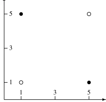
3.4 Demonstration of Non-Linearity
When the XOR function is scaled by4and shifted
by 1 unit along the x and y axes, the resultant
function maps the tuples (x = 5, y = 5) and
(x= 1, y = 1)to0and the tuples(x= 5, y = 1)
and(x= 1, y= 5)to1as shown in Figure 1.
We can verify by observation that the convex hulls around the data points in each of the cate-gories intersect. The convex hull around category
1is the line between{5,1}and{1,5}. The convex
hull around category0 is the line between{1,1}
and {5,5}. These lines intersect at {3,3}, and therefore the categories are not linearly separable. Since the categories are not linearly separable, if a classifier is capable of learning (correctly clas-sifying the points of) this XOR function it must be a non-linear classifier.
In this subsection, we demonstrate
experi-mentally that a 3-layer multinomial hierarchical
Bayesian classifier with a “sum-of-products”
pos-terior and4 hidden nodes (2 per class) can learn
this function.
Figure 2 shows the outputs of various classifiers trained on the XOR function described in Figure 1 when run on random points in the domain of the
-6
1 3 5
1 3 5
e
e u
u
Figure 1: A 2-D plot of the shifted and scaled XOR function, where the filled circles stand for
points that map to 1 and the unfilled circles for
points that map to0.
function. The small dots were placed at all points classified as1.
3.4.1 Naive Bayes
It can be seen from Figure 2a that the boundary learnt by the naive Bayes classifier is a straight line through the origin.
It can be seen that no matter what the angle of the line is, at least one point of the four will be misclassified.
In this instance, it is the point at{5,1} that is
misclassified as 0 (since the clear area represents
the class0).
3.4.2 Multinomial Non-Linear Hierarchical Bayes
The decision boundary learnt by a multinomial
non-linear hierarchical Bayes classifier (one that computes the posterior using a sum of products of the hidden-node conditional feature probabilities) is shown in Figure 2b.
The boundary consists of two straight lines passing through the origin. They are angled in such a way that they separate the data points into the two required categories.
All four points are classified correctly since the points at {1,1} and {5,5} fall in the clear
con-ical region which represents a classification of 0
whereas the other two points fall in the dotted
re-gion representing class1.
Therefore, we have demonstrated that the multi-nomial non-linear hierarchical Bayes classifier can learn the non-linear function of Figure 1.
[image:6.612.325.502.43.212.2](a) Naive Bayes
(b) Multinomial Non-Linear Hierarchical Bayes
(c) Gaussian Non-Linear Hierarchical Bayes
Figure 2: Decision boundaries learnt by classi-fiers trained on the XOR function of Figure 1. The dotted area represents what has been learnt as the
category1. The clear area represents category0.
3.4.3 Gaussian Non-Linear Hierarchical Bayes
The decision boundary learnt by aGaussian
[image:7.612.95.291.45.652.2]non-linear hierarchical Bayes classifier is shown in Figure 2c.
The boundary consists of two quadratic curves separating the data points into the required cate-gories.
Therefore, the Gaussian non-linear hierarchical Bayes classifier can also learn the function de-picted in Figure 1.
Thus, we have demonstrated that3-layer
hierar-chical Bayesian classifiers (multinomial and
Gaus-sian) with a “sum-of-products” posterior and 4
hidden nodes (2 per class) can learn certain
non-linear functions.
3.5 Intuition on Learning Arbitrary Non-Linear Functions
Non-linear hierarchical Bayesian models based on the multinomial distribution are restricted to hy-perplanes that pass through the origin. Each hid-den node represents a linear boundary passing through the origin. Models based on the Gaus-sian distribution are not so restricted. Each hidden node in their case is associated with a quadratic boundary.
Assuming that the hidden nodes act as cluster centroids and fill the available hyperspace of a given class (for a suitable probability distribution), one might expect the dominance of the closest hid-den nodes - dominance of one hidhid-den node for text datasets is likely on account of extreme posterior probabilities (Eyheramendy et al, 2003) - to re-sult in the piece-wise reconstruction of arbitrary boundaries in the case of Gaussian models. The dominance of the nearest hidden nodes (in terms of angular distances) is likely to result in appro-priate radial boundaries in the case of multinomial models.
We now demonstrate empirically that a classi-fier capable of learning non-linear boundaries can outperform linear classifiers on certain text and tu-ple classification tasks.
4 Experimental Results
the last, the Gaussian version was used.
With both the naive Bayes classifier and the hi-erarchical Bayesian models, the smoothing used was Laplace smoothing. The SVM classifier used a linear kernel.
4.1 Large Movie Review Dataset
The first experiment was run on the large movie review dataset (Maas et al, 2011) which consists of
50,000movie reviews labelled as either positive
or negative (according to whether they expressed positive or negative sentiment about a movie).
The training set size was varied between5,000
and 35,000 in steps of 5,000 (with half the
re-views drawn from positively labelled data and the other half drawn from negatively labelled data).
Of the remaining data, we used 5,000 reviews
(2,500 positive and2,500negative) as a
valida-tion set. The rest were used as test data.
The accuracies for different training set sizes and hidden nodes are as shown in Figure 3. The
accuracies obtained when training on25,000
re-views and testing on20,000(with the remaining
5000documents of the test set used for validation)
are shown in Table 1 .
Classifier Accuracy
Naive Bayes 0.7964±0.0136
MaxEnt 0.8355±0.0149
SVM 0.7830±0.0128
[image:8.612.312.518.33.535.2]Non-linear Hierarchical Bayes 0.8438±0.0110
Table 1: Accuracy on the movie reviews dataset when trained on 25,000 reviews.
4.2 Single-Label Text Categorization Datasets
We tested the performance of the various classi-fiers (the hierarchical Bayes classifier was
con-figured with 2 hidden nodes per class) on the
Reuters R8, R52 and 20 Newsgroups datasets preprocessed and split as described in
(Cardoso-Cachopo, 2007).10%of the training data was held
back for validation. The results are shown in Ta-ble 2.
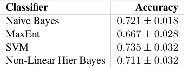
4.3 Query Classification Dataset
For this experiment, we used a smaller corpus of
1889queries classified into14categories (Thomas
Morton, 2005). Five different random orderings of
5 10 15 20 25 30 35
0.75 0.8 0.85 0.9
1000s of training reviews
Accurac
y
Naive Bayes
Non-Linear Hierarchical Bayes MaxEnt
SVM A
5 10 15 20 25 30 35
0.8 0.85 0.9
1000s of training reviews
Accurac
y
1 hidden node per class 2 hidden nodes per class 3 hidden nodes per class 4 hidden nodes per class 5 hidden nodes per class B
0 10 20
0.5 0.6 0.7 0.8 0.9
100s of training reviews
Accurac
y
Naive Bayes MaxEnt SVM
Non-Linear Hierarchical Bayes C
Figure 3: Evaluations on the movie reviews
dataset. Plot A shows the performance of vari-ous classifiers on the dataset (the multinomial non-linear hierarchical Bayes classifier being
config-ured with2hidden nodes per class and trained
us-ing 50 repetitions of 4 iterations of soft
expecta-tion maximizaexpecta-tion). Plot B compares the accura-cies of multinomial non-linear hierarchical Bayes classifiers with different numbers of hidden nodes. Plot C charts the performance of the classifiers on much smaller quantities of data than in plot A (the
2-hidden-node multinomial non-linear
hierarchi-cal Bayes classifier being trained with 10
repeti-tions of5expectation maximization iterations).
Classifier R8 R52 20Ng
Naive Bayes 0.955 0.916 0.797
MaxEnt 0.953 0.866 0.793
SVM 0.946 0.864 0.711
Non-Lin Hier Bayes 0.964 0.921 0.808
[image:9.612.87.300.40.107.2]Table 2: Accuracy on Reuters R8, R52 and 20 Newsgroups.
Figure 4: Artificial2-dimensional dataset: a) ring
b) dots c) XOR d) S
the data in the corpus were used, each with1400
training,200validation and289test queries.
The accuracies of different classifiers (including
a hierarchical Bayes classifier with4hidden nodes
per class trained through50repetitions of10
iter-ations of expectation maximization) on the query dataset are as shown in Table 3. The error margins are large enough to render all comparisons on this dataset devoid of significance.
Classifier Accuracy
Naive Bayes 0.721±0.018
MaxEnt 0.667±0.028
SVM 0.735±0.032
Non-Linear Hier Bayes 0.711±0.032
Table 3: Accuracy on query classification.
4.4 Artificial2-Dimensional Dataset
A total of2250points were generated at random
positions(x, y)inside a square of width500.
Those falling inside each of the four shaded
shapes shown in Figure 4 were labelled 1and the
rest of the points (falling outside the shaded areas
of the square) were labelled0.
For each shape,1000of the points were used for
training,250as the validation set and the
remain-ing 1000 as the test set. Naive Bayes and
non-linear hierarchical Bayes classifiers that assumed the Gaussian distribution were used.
The Gaussian naive Bayes (GNB) classifier and the non-linear Gaussian hierarchical Bayes (GHB)
classifier (10hidden nodes per class), trained with
10 repetitions of 100 iterations of expectation
maximization were tested on the artificial dataset. Their accuracies are as shown in Table 4.
Shape GNB GHB
ring 0.664 0.949
dots 0.527 0.926
XOR 0.560 0.985
[image:9.612.98.287.175.387.2]S 0.770 0.973
Table 4: Accuracy on the artificial dataset.
4.5 Discussion
We see from Table 1 that the multinomial non-linear hierarchical Bayes classifier significantly outperforms the naive Bayes and SVM classifiers on the movie reviews dataset. We see from Ta-ble 2 that its performance compares favourably with that of other classifiers on the Reuters R8, the Reuters R52 and the 20 Newsgroups datasets.
We also observe from Plot B of Figure 3 that multinomial non-linear hierarchical Bayes
classi-fiers with2,3,4and5hidden nodes outperform1
hidden node on that dataset.
Finally, we observe that the artificial dataset is modeled far better by a Gaussian non-linear hier-archical Bayes classifier than by a Gaussian naive Bayes classifier.
5 Conclusions
We have shown that generative classifiers with a hidden layer are capable of learning non-linear decision boundaries under the right conditions (independence assumptions), and therefore might
be said to be capable of deep learning. We
have also shown experimentally that multinomial non-linear hierarchical Bayes classifiers can out-perform some linear classification algorithms on some text classification tasks.
[image:9.612.368.481.247.320.2] [image:9.612.95.284.577.647.2]References
Aixin Sun and Ee-Peng Lim. 2001. Hierarchical Text Classification and Evaluation. InProceedings of the 2001 IEEE International Conference on Data Min-ing, ICDM ’01, 521–528.
Andrew L. Maas, Raymond E. Daly, Peter T. Pham, Dan Huang, Andrew Y. Ng, and Christopher Potts. 2011. Learning Word Vectors for Sentiment Anal-ysis. InProceedings of the 49th Annual Meeting of the Association for Computational Linguistics: Hu-man Language Technologies, ACL-HLT2011, 142– 150.
Alex Krizhevsky, and Geoffrey E. Hinton. 2011. Us-ing very deep autoencoders for content-based image retrieval.ESANN.
Alexandr Andoni, Rina Panigrahy, Gregory Valiant, and Li Zhang. 2014. Learning polynomials with neural networks. ICML.
Ana Cardoso-Cachopo. 2007. Improving Methods for Single-label Text Categorization. PhD Thesis, Insti-tuto Superior Tecnico, Universidade Tecnica de Lis-boa.
Asja Fischer and Christian Igel. 2012. An Introduction to Restricted Boltzmann Machines.Progress in Pat-tern Recognition, Image Analysis, Computer Vision, and Applications, 17th Iberoamerican Congress, CIARP 2012, Buenos Aires, Argentina, September 3-6, 2012. Proceedings, 7441:14–36.
Andrew Y. Ng and Michael I. Jordan. 2001. On dis-criminative vs. generative classifiers: A compari-son of logistic regression and naive bayes. In Ad-vances in Neural Information Processing Systems 14 (NIPS’01), 841–848.
Arthur P. Dempster, Nan M. Laird, and Donald B. Ru-bin. 1977. Maximum likelihood from incomplete data via the EM algorithm.Journal of the royal sta-tistical society. Series B (methodological). 1–38. JS-TOR.
Chuong B. Do, and Serafim Batzoglou. 2008. What is the expectation maximization algorithm?. Na-ture biotechnology. 26(8):897-899. Nature Publish-ing Group.
Daphne Koller and Nir Friedman. 2009. Probabilistic graphical models: principles and techniques. MIT Press, Cambridge, MA.
David E. Rumelhart, Geoffrey E. Hinton, and R. J. Williams. 1986. Learning Internal Representations by Error Propagation. In Parallel distributed pro-cessing: explorations in the microstructure of cog-nition. 1:318-362. MIT Press, Cambridge, MA.
David H. Ackley, Geoffrey E. Hinton, Terrence J. Se-jnowski. 1985. A learning algorithm for Boltzmann machines. InCognitive science. 9(1):147-169.
George Cybenko. 1989. Approximation by superpo-sitions of a sigmoidal function. InMathematics of control, signals and systems. 2(4):303–314
Hao Wang and Dit-Yan Yeung. 2016. Towards Bayesian Deep Learning: A Survey.CoRR. Martin J.Wainwright and Michael I. Jordan. 2008.
Graphical models, exponential families, and varia-tional inference. Foundations and TrendsR in
Ma-chine Learning, 1(1-2):1–305.
Marvin Minsky and Seymour Papert. 1988. Percep-trons: an introduction to computational geometry (expanded edition). MIT Press, Cambridge, MA. Michael I. Jordan, and Chris Bishop. 2004. An
intro-duction to graphical models. Progress.
Miguel E. Ruiz, and Padmini Srinivasan. 2002. Hierar-chical Text Categorization Using Neural Networks. InInformation Retrieval, 5(1):87–118.
Nan Laird, Nicholas Lange, and Daniel Stram. 1987. Maximum likelihood computations with repeated measures: application of the EM algorithm.Journal of the American Statistical Association, 82(397):97– 105.
Paul Smolensky. 1986. Chapter 6: Information Pro-cessing in Dynamical Systems: Foundations of Har-mony Theory. Parallel Distributed Processing: Ex-plorations in the Microstructure of Cognition, Vol-ume 1: Foundations, 1:194281. MIT Press, Cam-bridge, MA.
Susana Eyheramendy, David D. Lewis, and David Madigan. 2003. On the Naive Bayes Model for Text Categorization. In9th International Workshop on Artificial Intelligence and Statistics.
Thomas Morton. 2005. Using semantic relations to improve information retrieval. Dissertations avail-able from ProQuest. Paper AAI3197718.
Qinpei Zhao, Ville Hautamaki, and Pasi Franti. 2011. RSEM: An Accelerated Algorithm on Repeated EM.
2011 Sixth International Conference on Image and Graphics (ICIG). IEEE.
Shivakumar Vaithyanathan, Jianchang Mao, and Byron Dom. 2000. Hierarchical Bayes for Text Classifi-cation. PRICAI Workshop on Text and Web Mining, 36-43.
Sriharsha Veeramachaneni, Diego Sona, and Paolo Avesani. 2005. Hierarchical Dirichlet Model for Document Classification. In Proceedings of the 22Nd International Conference on Machine Learn-ing, ICML ’05, 928–935.
Yann LeCun, Yoshua Bengio, and Geoffrey Hinton. 2015. Deep learning.Nature, 521:436-444. Yoshua Bengio. 2009. Learning deep architectures for
AI. Foundations and trends in Machine Learning, 2(1):1-127.
Zhibin Liao and Gustavo Carneiro. 2015. The use of deep learning features in a hierarchical classifier learned with the minimization of a non-greedy loss function that delays gratification. 2015 IEEE In-ternational Conference on Image Processing (ICIP), IEEE.