NCSU_SAS_SAM: Deep Encoding and Reconstruction
for Normalization of Noisy Text
Samuel P. Leeman-Munk James C. Lester
Center for Educational Informatics
North Carolina State University
Raleigh, NC, USA
{spleeman, lester}@ncsu.edu
James A. Cox
Text Analytics R&D
SAS Institute Inc.
Cary, NC, USA
[email protected]
Abstract
As a participant in the W-NUT Lexical Normalization for English Tweets chal-lenge, we use deep learning to address the constrained task. Specifically, we use a combination of two augmented feed forward neural networks, a flagger that identifies words to be normalized and a normalizer, to take in a single token at a time and output a corrected version of that token. Despite avoiding off-the-shelf tools trained on external data and being an entirely context-free model, our sys-tem still achieved an F1-score of 81.49%, comfortably surpassing the next runner up by 1.5% and trailing the second place model by only 0.26%.
1
Introduction
The phenomenal growth of social media, web forums, and online reviews has spurred a grow-ing interest in automated analysis of user-generated text. User-user-generated text presents sig-nificant computational challenges because it is often highly disfluent. To address these chal-lenges, we have begun to see a growing demand for tools and techniques to transform noisy user-generated text into a canonical form, most re-cently in the Workshop on Noisy User Text at the Association for Computational Linguistics. This work describes a submission to the Lexical Normalization for English Tweets challenge as part of this workshop (Baldwin et al., 2015)
Motivated by the success of prior deep neural network architectures, particularly denoising au-toencoders, we have developed an approach to transform noisy user-generated text into a canon-ical form with a feed-forward neural network augmented with a projection layer (Collobert et al., 2011; Kalchbrenner, Grefenstette, & Blunsom, 2014; Vincent, Larochelle, Bengio, & Manzagol, 2008). The model performs a charac-ter-level analysis on each word of the input. The absence of hand-engineered features and the avoidance of direct and indirect external data make this model unique among the three top-performing models in the constrained task.
This paper is organized as follows. In Sec-tion 2 we describe each component of our model. In Section 3 we describe the specific instantia-tion of our model, and in Secinstantia-tion 4 we present and discuss results.
2
Architecture and Components
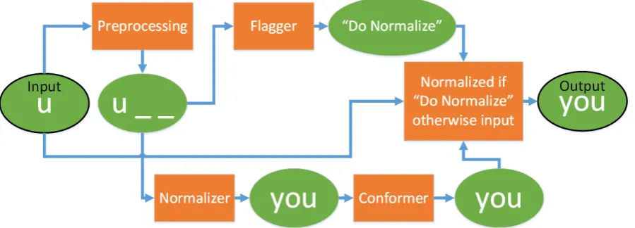
Our model consists of three components: a Nor-malizer that encodes the input and then recon-structs it in normalized form, a Flagger that de-termines whether the Normalizer should be used or if the word should be taken as-is, and a Con-former that attempts to smooth out simple errors introduced by quirks in the Normalizer.
In this section we will use the simple example transformation of “u” to “you” where “u” is the input text and “you” is the gold standard normal-ization. In our example we use a maximum word size of three. Figure 1 shows the flow of our ex-ample through the model. In broad overview, the input is preprocessed and sent to both the
malizer and the Flagger. The Normalizer com-putes a candidate normalization, and the Flagger determines whether to use that candidate or the original word. The Normalizer’s output is passed to the Conformer, which conforms it to a word in the vocabulary list, and then the candidate, the flag, and the original input word are passed to a simple decision component that either keeps the original word or uses the normalized version based on the output of the Flagger. While it may seem inefficient that the normalized version is always computed, even if it is not used, this ap-proach is used so that the Normalizer and Flag-ger can be run in parallel on many inputs at once.
2.1 Deep Feed-Forward Neural Networks As the central element of the Flagger and the Normalizer, the deep feed-forward neural net-work forms the basis of our model. A deep feed-forward neural network takes a vector of num-bers as input. This vector is known as a layer and each value within it is a neuron. The network
multiplies the input layer by a matrix of weights to return another vector. This new vector is then transformed by a non-linearity. A number of functions can serve as the non-linearity, includ-ing the sigmoid and the hyperbolic tangent, but our model uses a rectified linear unit, given by the following expression.
𝑦=max 𝑥,0
The rectified linear unit has been successful in a number of natural language tasks such as speech processing (Zeiler et al., 2013), and it was effec-tive in an unpublished part-of-speech tagging model we developed.
The transformed vector is referred to as a hid-den layer because its values are never directly observed in the normal functioning of the model.
A deep feed-forward neural network can contain any number of hidden layers, each going through the same process, multiplying by a matrix of weights and transforming via a non-linearity. Hidden layers may also be of any size. Multiple applications of learnable weight matrices and non-linear transformations together allow a deep neural network to represent complex relation-ships between input and output (Bengio, 2009).
Deep feed-forward neural networks are trained by backpropagation. Backpropagation is a train-ing method by which the gradient of any given weight in a network can be calculated from the error between the output of the network and a gold standard. It is described in more detail in (Rumelhart, Hinton, & Williams, 1986).
2.2 The Normalizer
Our use of deep feed-forward neural networks for the task of normalization is inspired by the success of denoising autoencoders. (Vincent et al., 2008). Denoising autoencoders are neural
networks whose output is the same as their input. That is, they specialize in developing a robust encoding of an input such that the input can be reconstructed from the encoding alone. The de-noising aspect refers to the fact that to encourage robustness, denoising autoencoders are given inputs that have been deliberately corrupted, or “noised” and are expected to reconstruct them without the noise. It is this “denoising” aspect that makes denoising autoencoders so interesting for text normalization.
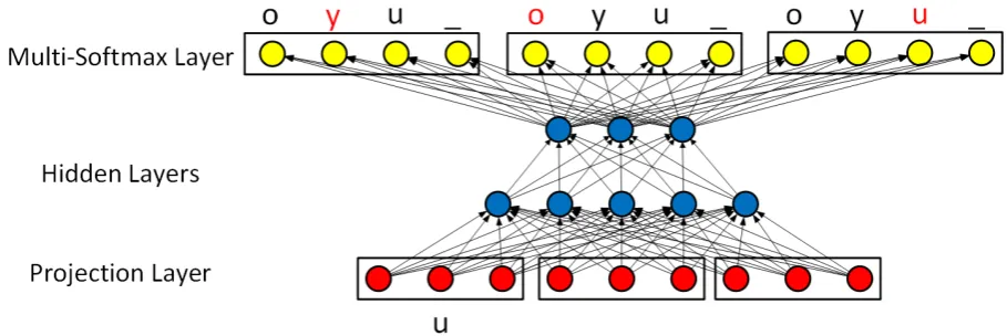
[image:2.595.74.524.360.522.2]internally, outputting the denoised (normalized) version. It accomplishes this in three sets of lay-ers. First the character projection layer takes a string and represents it as a fixed-length numeric vector. Next, a feed-forward neural network con-verts the data into its internal representation and, with a special output layer, into a denoised ver-sion of the input. Figure 2 shows a diagram of the Normalizer’s architecture.
The first step of the Normalizer is performed by the character projection layer (Collobert et al., 2011). The character projection layer learns floating point vector representations of charac-ters, which it concatenates into one large floating point vector word representation. In our example, the letter “u” is represented by n floating point numbers. For example, if n = 3 the representation for “u” might be [0.1, -1.2, -0.3]. This vector was chosen arbitrarily, but in the actual model, values are learned in training. The representations allow more information to be associated with a charac-ter than a simple numeric index.
In this simple example, the word “u” is com-posed of one character, but if it were longer, each letter would be separately represented. A key challenge at this point is that a feed-forward neu-ral network cannot handle an arbitrary number of inputs. Because each position in the vector is a neuron matched directly to a set of weights, changing the size of the vector would require changing the size of the learned weights, and the model would have to be retrained.
To accommodate this, we use a fixed window. Before we send our input to the Normalizer, we
preprocess it to meet a specified length, filling in unused spaces with a sentinel padding “charac-ter” that projects to its own set of learned weights like the other characters. Since the max-imum word size in our example is 3, we use a window of size 3. Therefore, our input “u”
be-comes [u, _, _] and then is projected and concatenated and becomes something like [0.1, 1.2, -0.3, 1.3, 0.0, -1.1, 1.3, 0.0, -1.1]. Notice that we have nine values now in our input. That is the three values from “u” and then the three values for “_” ([1.3, 0.0, -1.1]) twice, once for each “_”. After this step, the system has a numeric vector representation of a word that is always the same length. It now sends it to the first layer of the feed-forward neural network. We deliberately select a large enough window that only in a small minority of cases does a word have to be reduced to fit into the window.
The last hidden layer’s values go through one final matrix multiplication to output a list of val-ues wv in size, where w is the size of the window and v is the number of possible characters includ-ing the paddinclud-ing character, that is, the number of characters in the alphabet, which is shared be-tween the input and output layers. In this last layer the nonlinear transformation is a special version of the softmax operation.
The softmax operation transforms a vector such that each of its values is between zero and one and the new vector sums to one. Mathemati-cally, it is given as:
𝜎 𝑧 ! = 𝑒!"
𝑒!" !
!!!
Where K is the number of values in the vector. In our model, K = v, the size of the alphabet. These individual values can alternately be considered posterior probabilities for each of the possible decisions. If each value is mapped to a character,
[image:3.595.70.525.509.661.2]highest value in each of the w sets, but in training we take the whole prediction distribution and try to maximize the likelihood of each correct letter. We do not attempt to predict character embed-dings because we are learning them, and the model would be likely to learn a trivial function with character embeddings that are all equal.
Training the Normalizer as a whole relies on generating posterior distributions and attempting to minimize the total negative log likelihood of the gold standard. Mathematically, our objective function is
cost=− 𝑙𝑛 𝑝
!∈!
Where p is an element in P, the vector of the probabilities of each gold standard letter. So, if our model predicts “y” as 75% likely for charac-ter 1, “o” as 95% likely for characcharac-ter 2, and “u” as 89% likely for character 3 in our window of size 3, the negative log likelihoods calculated as (.29, .05, .12) are summed to get the error. This sum error gives a simple measurement of per-formance to optimize, which backpropagates through the model to learn all the weights de-scribed above (Rumelhart et al., 1986).
2.3 The Flagger
The Flagger identifies what does and does not require normalization. The vast majority of the training data (91%) does not require normaliza-tion, so returning the reconstructed encoding of every word would risk incorrectly regenerating an already canonical token.
The Flagger has the same general structure as the Normalizer itself except for the final layer. Instead of generating text at the last layer, a softmax layer predicts whether the token should be normalized at all. Thus, the Flagger’s output layer is two neurons in size, one representing the flag “Do Normalize,” and another representing the flag “Do Not Normalize.” In the construction of the gold standard for the task, there were three reasons a token would not be normalized: firstly, the token is already correct, second, the token is in a protected category (hashtags or foreign words), or third, it was simply unrecognizable such that the human normalizer could not find the correct form. The Flagger accounts for but does not distinguish between these three possibil-ities.
2.4 The Conformer
Even when a token should be corrected, it is pos-sible that the normalizer will come very close to
correcting it without succeeding. Reconstructing the word “laughing,” for instance, the normalizer can fail completely if it predicts even one letter wrong. An early analysis of validation data found that the normalizer had predicted “laugling” in-stead of laughing. These off-by-one errors are a frequent enough occurrence to merit a module to deal with them. The Conformer is also useful for correctly normalizing rare words whose correct normalization is too long for the window to rep-resent. In particular “lmfao” expands to an im-pressive 27 characters, but if the Normalizer pre-dicts only the first 25 characters, the Conformer can easily select the correct token.
To correct these small normalizer errors we construct the Conformer by collecting a diction-ary from the gold standard training data. The dic-tionary is simply a list of all the unique words in the gold standard data. Then at runtime, whenev-er the Normalizwhenev-er runs and predicts a word that is not present in the dictionary, we replace it with the closest word in the dictionary according to Levenshtein distance (Levenshtein, 1966). Ties are resolved based on which word comes first in the dictionary. Because Python’s set function, which does not guarantee a specific order of its contents, is used to construct the dictionary, the dictionary’s order is not predictable and thus ties are resolved unpredictably.
3
Settings and Evaluation
layer. Dropout has been shown to improve per-formance by discouraging overfitting on the training data, and 50% and 75% are common dropout rates (Hinton, 2014).
We found the highest F1 score on the valida-tion data for the Normalizer with two hidden lay-ers of size 2000 each and 50% dropout. This was close to the maximum size our GPU could sup-port without reducing the batch size to be too small to take advantage of the parallelism. The Flagger’s highest score was found at two hidden layers of size 1000 each and 75% dropout. At-tempts to provide hidden layers of different sizes consistently found inferior results. For the size of each embedding in the character projection layer, 10 had proven effective earlier in a simpler un-published Twitter part-of-speech task. We select-ed 25 for our character embselect-edding size to ac-count for the greater complexity of a normaliza-tion task.
We separated the provided training data into 90% training data, 5% validation data and 5% was held out as test data. In order to construct a useful model on the small amount of available data, we iterate training over the same data many times. Our model stopped training after 150 training iterations in which there was no im-provement on the validation set. We chose 150 iterations as the smallest value that did not lead to ending the training at a clearly suboptimal value. The training also stops at 5,000 iterations but in practice it converged before reaching this value.
Early in development we found that the Nor-malizer had exceptional trouble reconstructing twitter-specific objects, that is, hash-tags (#goodday), at-mentions (@marysue) and URLs (http://blahblah.com). Generally its behavior in all three cases was to follow the standard marker characters (@, #, http://) with a string of gibber-ish unrelated to the word itself. Because these are protected categories that should not be changed, we removed them from the training data and rely on the Flagger to flag them as not to be correct-ed.
We used layer-wise pre-training, meaning we first trained with zero hidden layers (going di-rectly from the character projection to the soft-max layer) to initialize the character embeddings, then we trained with one hidden layer, initializ-ing the character embeddinitializ-ings with their previ-ously trained values. When we trained the full model using two hidden layers, we initialized both the character projection layer and the weights from the projected input to the first
hid-den layer with the values learned before. The model continued to learn all the weights it used. Pretrained weights continued to be trained in the full model, although “freezing” some pretrained weights after pretraining and only training later weights in the full model has shown success when working with large amounts of unsuper-vised data and may be worthwhile to consider in future work (Yosinski, Clune, Bengio, & Lipson, 2014).
Running on an NVIDIA GeForce GTX 680 GPU with 2 GB of onboard memory, training the Normalizer took about six hours. We do not in-clude CPU and RAM specifications because they were not heavily utilized in the GPU implemen-tation. The Flagger was considerably faster to train than the Normalizer, taking only a little over half an hour.
4
Results and Discussion
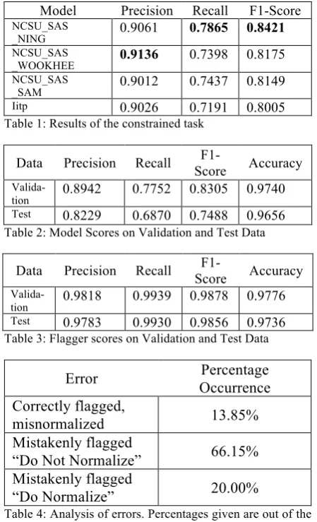
The model earned third place in the competition, with scores very close to the second place model. The model’s results in the competition compared to the first, second, and fourth place models is shown in Table 1. The precision scores are much higher than the recall scores for all models be-cause in this task precision measures the capabil-ity of the model to not normalize what does not need normalizing while recall requires that a model both correctly identify what needs to be normalized and correctly normalize it.
In addition to the challenge results, we per-formed a more in-depth analysis on our own held-out validation and test data. Our analysis of the scores is shown in Table 2.
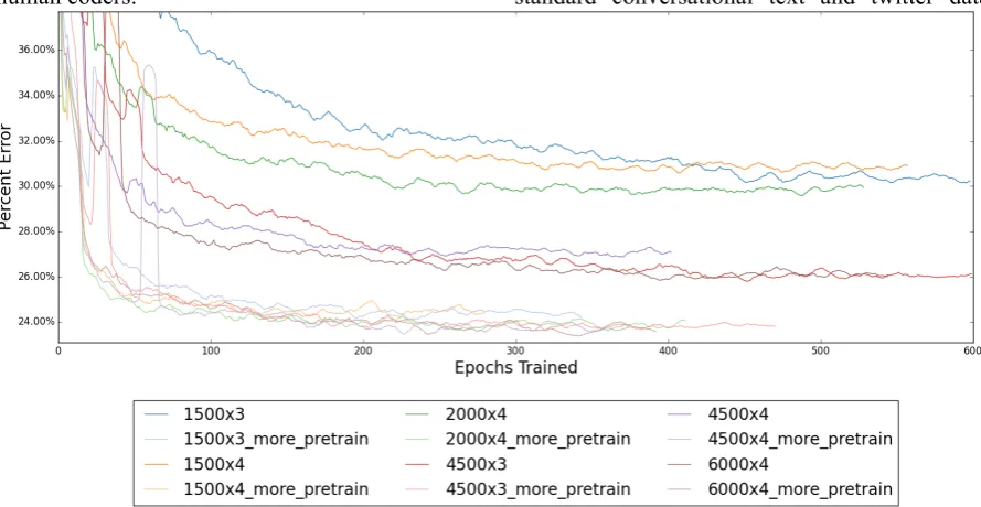
percent. We show this graph to illustrate a num-ber of points. Particularly, we wish to illustrate the challenge of encoding and reconstructing every item in a massive vocabulary, the value of additional iterations of layer-wise pre-training, and the large spikes in the error rates at certain points in the model.
Model Precision Recall F1-Score NCSU_SAS
_NING 0.9061 0.7865 0.8421
NCSU_SAS
_WOOKHEE 0.9136 0.7398 0.8175
NCSU_SAS
_SAM 0.9012 0.7437 0.8149
Iitp 0.9026 0.7191 0.8005
Table 1: Results of the constrained task
Data Precision Recall
F1-Score Accuracy
Valida-tion 0.8942 0.7752 0.8305 0.9740
Test 0.8229 0.6870 0.7488 0.9656
Table 2: Model Scores on Validation and Test Data
Data Precision Recall Score F1- Accuracy
Valida-tion 0.9818 0.9939 0.9878 0.9776
Test 0.9783 0.9930 0.9856 0.9736
Table 3: Flagger scores on Validation and Test Data
Error Occurrence Percentage Correctly flagged,
misnormalized 13.85%
Mistakenly flagged
“Do Not Normalize” 66.15% Mistakenly flagged
[image:6.595.68.293.171.541.2]“Do Normalize” 20.00%
Table 4: Analysis of errors. Percentages given are out of the total error count.
Original Gold
Stand-ard Normalized
FB Facebook fabol
Fuhh f*** fuhh
OPENFOLLOW open follow openffolow
Feela Feels feela
Bkuz because bkuze
Kin kind of kin
Bruuh brother bruuhr
Table 5: Examples of tokens that were mistakenly flagged "Do Not Normalize.” The “Normalized” column is what the model would have produced if the Flagger had produced the flag “Do Normalize”
The Normalizer demands much more
rep-resentational power when not assisted by the
Flagger. Before we added the Flagger, we
saw continual improvement of results going
up to four layers of six thousand nodes each.
We saw greater improvements from adding
more nodes per layer than from adding more
layers. The cluster of three lines near the top
all have layers of 1500 or 2000 nodes each,
and the next cluster down is the models we
tried with 4500 and 6000 nodes. Incidentally,
all but the smallest of these models were too
large for our GPU’s 2GB of onboard
memory. As a reminder, after we added the
flagger, we only required two layers of 2000
nodes each to get competitive results. In each
case we used a dropout rate of 50%.
The default models pre-trained each layer for 250 iterations and we also trained models with the same structure for 500 iterations. We find a noticeable improvement in the error rate for the models that were pre-trained for more iterations. In the graph, the models with more pre-training make up the cluster of lines near the bottom of the graph.
Looking at the graphs, one may notice that some lines have brief spikes multiple percentage points in size. Because it only takes a one-letter mistake for a word to be misnormalized, we ex-pect that at these times a small error arose that affected a large number of words. It is worth pointing out that each model continues to im-prove while in its spike, eventually dropping back to pre-spike levels.
The model is unique among the three top-performing models in that it avoids external data both directly and through indirect sources. The constrained task does not allow external data, but it does allow the use of off-the-shelf tools trained on external data. Our model does not use any such tools. Without the assistance of tools such as part-of-speech taggers, attempts to use context proved ineffective, likely because of increased sparsity. A given word that appears in the train-ing set three hundred times may only appear three times after another particular word, and may not occur more than once with a particular prior word and following word, so it is more dif-ficult to find patterns in limited data. Future work could either attempt to use tools to provide additional information or could simply take ad-vantage of large amounts of data to learn directly the relationships such tools traditionally abstract for the benefit of conventional machine learning.
[image:6.595.71.291.561.675.2]exam-ple, sometimes the word “pics” used to refer to pictures was normalized to “pictures” but other times it was left as “pics”. These inconsistencies in the gold standard make it difficult to accurate-ly judge the quality of the models submitted. Oc-casionally when we examined mistakes the mod-el made, we found that the modmod-el’s prediction was correct according to the gold standard, but that the gold standard was wrong. An inter-rater reliability measure would help us to gauge not only how well our models compare to each other but how they compare to agreement between human coders.
5
Conclusions and Future Work
Normalization of Twitter text is a challenging task. With a direct application of simple deep learning techniques and without relying on any sources of external data, direct or indirect, we built a model that performed competitively with the other models in the task. Our method shows the ability of deep learning to tackle complex tasks without labor-intensive hand-engineering of features.
An important direction for future work is sim-plifying the normalization pipeline. The need for a Conformer in particular suggests that there is room for improvement in the model. Although constructing the normalized form rather than se-lecting from a list leaves the possibility open that a system could normalize to a correct word that did not appear in the training data, in practice
this happened much less often than having the system normalize incorrectly. A model that pre-dicts words from a vocabulary instead of recon-structing them would be faster to train and would not require a Conformer, and, considering the top two models were vocabulary based, might out-perform our reconstruction-based model.
A second direction for future work centers on leveraging external data. With more time and greater computing power, it may be the case that it is possible to learn sophisticated language models in an unsupervised fashion from both standard conversational text and twitter data.
With this additional data, a model may be able to effectively use context in distinguishing between multiple possible normalizations of a word. De-noising autoencoders in particular are known to make good use of unsupervised data.
A third direction for future work is to investi-gate more challenging normalization tasks that include correction of syntax and do not present the text already tokenized. These will give us an opportunity to attempt tasks closer to the chal-lenges our normalization systems will face in the real world.
[image:7.595.73.518.231.461.2]would lose the emphasis implied by the elonga-tion of the vowel. For some tasks, it may be im-portant to retain the information contained in such non-canonical forms.
References
Baldwin, Timothy, Catherine, Marie, Han, Bo, Kim, Young-Bum, Ritter, Alan, & Xu, Wei. (2015). Shared Tasks of the 2015 Workshop on Noisy User-generated Text : Twitter Lexical
Normalization and Named Entity Recognition. In
Proceedings of the Workshop on Noisy User-generated Text (WNUT 2015). Beijing, China.
Bastien, Frédéric, Lamblin, Pascal, Pascanu, Razvan, Bergstra, James, Goodfellow, Ian, Bergeron, Arnaud, … Bengio, Yoshua. (2012). Theano: New Features and Speed Improvements. In Deep Learning and Unsupervised Feature Learning NIPS 2012 Workshop (pp. 1–10). Retrieved from http://arxiv.org/abs/1211.5590v1
Bengio, Yoshua. (2009). Learning Deep Architectures for AI. Foundations and Trends® in Machine Learning, 2(1), 1–127.
http://doi.org/10.1561/2200000006
Bergstra, James, Breuleux, Olivier, Bastien, Frédéric, Lamblin, Pascal, Pascanu, Razvan, Desjardins, Guillaume, … Bengio, Yoshua. (2010). Theano: A CPU and GPU Math Compiler in Python. In
Proceedings of the 9th Python in Science Conference (pp. 3–10). Austin, Texas.
Collobert, Ronan, Weston, Jason, Bottou, Leon, Karlen, Michael, Kavukcuoglu, Koray, & Kuksa, Pavel. (2011). Natural Language Processing (almost) from Scratch. The Journal of Machine Learning Research, 12, 2493–2537. Retrieved from http://dl.acm.org/citation.cfm?id=2078186
Hinton, Geoffrey. (2014). Dropout : A Simple Way to Prevent Neural Networks from Overfitting. The Journal of Machine Learning Research, 15, 1929– 1958.
Kalchbrenner, Nal, Grefenstette, Edward, & Blunsom, Phil. (2014). A Convolutional Neural Network for Modelling Sentences. ACL, 655–665.
Levenshtein, Vladimir. (1966). Binary Codes Capable of Correcting Deletions, Insertions, and Reversals.
Soviet Physics Doklady, 10(8), 707–710.
Rumelhart, David, Hinton, Geoffrey, & Williams, Ronald. (1986). Learning Representations by Back-propagating Errors. Nature, 323(9), 533–
536. Retrieved from
http://books.google.com/books?hl=en&lr=&id=FJ blV_iOPjIC&oi=fnd&pg=PA213&dq=learning+re
presentations+by+back-propagating+errors&ots=zZEk5hHYWU&sig=B8 6wdYsAvCWVEN3aA-RCmw8_IJ8
Vincent, Pascal, Larochelle, Hugo, Bengio, Yoshua, & Manzagol, Pierre-antoine. (2008). Extracting and Composing Robust Features with Denoising Autoencoders. Proceedings of the 25th
International Conference on Machine Learning - ICML ’08, (July), 1096–1103.
http://doi.org/10.1145/1390156.1390294
Yosinski, Jason, Clune, Jeff, Bengio, Yoshua, & Lipson, Hod. (2014). How Transferable are Features in Deep Neural Networks? In Advances in Neural Information Processing Systems 27 (pp. 1–9).
Zeiler, M. D., Ranzato, M., Monga, R., Mao, M., Yang, K., Le, Q. V., … Hinton, G. E. (2013). On Rectified Linear Units for Speech Processing.
ICASSP, IEEE International Conference on Acoustics, Speech and Signal Processing - Proceedings, 3517–3521.