Learning Semantic Network Patterns for Hypernymy
Extraction
Tim vor der Br¨uck
Intelligent Information and Communication Systems (IICS) FernUniversit¨at in Hagen
Abstract
Current approaches of hypernymy ac-quisition are mostly based on syntactic or surface representations and extract hypernymy relations between surface word forms and not word readings. In this paper we present a purely se-mantic approach for hypernymy ex-traction based on semantic networks (SNs). This approach employs a set of patterns
sub0(a1, a2) ← premise where the premise part of a pattern is given by a SN. Furthermore this paper describes how the patterns can be derived by relational statistical learning following the Minimum Description Length prin-ciple (MDL). The evaluation demon-strates the usefulness of the learned patterns and also of the entire hyper-nymy extraction system.
1 Introduction
A concept is a hypernym of another concept if the first concept denotes a superset of the second. For instance, the class ofanimals is a superset of the class of dogs. Thus, animal is a hypernym of its hyponym dog and a hyper-nymy relation holds between animal and dog. A large collection of hypernymy (supertype) relations is needed for a multitude of tasks in natural language processing. Hypernyms are required for deriving inferences in ques-tion answering systems, they can be employed to identify similar words for information re-trieval or they can be useful to avoid word-repetition in natural language generation sys-tems. To build a taxonomy manually requires a large amount of work. Thus, automatic ap-proaches for their construction are preferable.
In this work we introduce a semantically ori-ented approach where the hypernyms are ex-tracted using a set of patterns which are nei-ther syntactic nor surface-oriented but instead purely semantic and are based on a SN for-malism. The patterns are applied on a set of SNs which are automatically derived from the German Wikipedia1 by a deep syntactico-semantic analysis. Furthermore, these pat-terns are automatically created by a machine learning approach based on the MDL princi-ple.
2 Related Work
Patterns for hypernymy extraction were first introduced by Hearst (Hearst, 1992), the so-called Hearst patterns. An example of such a pattern is:
NPhypo{,NPhypo}*{,} and other NPhyper.
These patterns are applied on arbitrary texts and the instantiated variables NPhypo
andNPhyper are then extracted as a concrete
hypernymy relation.
Apart from the handcrafted patterns there was also some work to determine patterns automatically from texts (Snow and others, 2005). For that, Snow et al. collected sen-tences in a given text corpus with known hy-pernym noun pairs. These sentences are then parsed by a dependency parser. Afterwards, the path in the dependency tree is extracted which connects the corresponding nouns with each other. To account for certain key words indicating a hypernymy relation likesuch (see first Hearst pattern) they added the links to the word on either side of the two nouns (if not yet contained) to the path too. Frequently
oc-1Note that for better readability the examples are
curring paths are then learned as patterns for indicating a hypernymy relation.
An alternative approach for learning pat-terns which is based on a surface instead of a syntactic representation was proposed by Morin et al. (Morin and Jaquemin, 2004). They investigate sentences containing pairs of known hypernyms and hyponyms as well. All these sentences are converted into so-called “lexico-syntactic expressions” where all NPs and lists of NPs are replaced by special sym-bols, e.g.: NP find in NP such as LIST. A similarity measure between two such expres-sions is defined as the sum of the maximal length of common substrings for the maxi-mum text windows before, between and after the hyponym/hypernym pair. All sentences are then clustered according to this similarity measure. The representative pattern (called
candidate pattern) of each cluster is defined to be the expression with the lowest mean square error (deviation) to all other expressions in the same similarity cluster. The patterns to be used for hyponymy detection are the can-didate patterns of all clusters found.
3 MultiNet
MultiNet is an SN formalism (Helbig, 2006). In contrast to SNs like WordNet (Fellbaum, 1998) or GermaNet (Hamp and Feldweg, 1997), which contain lexical relations between synsets, MultiNet is designed to comprehen-sively represent the semantics of natural lan-guage expressions. An SN in the MultiNet formalism is given as a set of vertices and arcs where the vertices represent the concepts (word readings) and the arcs the relations (or functions) between the concepts. A vertex can be lexicalized if it is directly associated to a lexical entry or non-lexicalized. An example SN is shown in Fig. 1. Note that each vertex of the SN is assigned both a unique ID (e.g.,
c2) and a label which is the associated lexical entry for lexicalized vertices andanonfor non-lexicalized vertices. Thus, two SNs differing only by the IDs of the non-lexicalized vertices are considered equivalent. Important Multi-Net relations/functions are (Helbig, 2006):
• agt: Conceptual role: Agent
• attr: Specification of an attribute
• val: Relation between a specific at-tribute and its value
• prop: Relation between object and prop-erty
• *itms: Function enumerating a set
• pred: Predicative concept characterizing a plurality
• obj: Neutral object
• sub0: Relation of conceptual subordi-nation (hyponymy) and hyperrelation to subr,subs, and sub
• subs: Relation of conceptual subordina-tion (for situasubordina-tions)
• subr: Relation of conceptual subordina-tion (for relasubordina-tions)
• sub: Relation of conceptual subordina-tion other than subsand subr
MultiNet is supported by a semantic lexicon (Hartrumpf and others, 2003) which defines, in addition to traditional grammatical entries like gender and number, semantic information consisting of one or more ontological sorts and several semantic features for each lexicon en-try. The ontological sorts (more than 40) form a taxonomy. In contrast to other taxonomies, ontological sorts are not necessarily lexical-ized, i.e., they need not denote lexical entries. The following list shows a small selection of ontological sorts which are inherited from ob-ject:
• Concrete objects: e.g.,milk,honey – Discrete objects: e.g., chair – Substances: e.g.,,milk,honey • Abstract objects: e.g., race,robbery
Semantic features denote certain semantic properties for objects. Such a property can either be present, not present or underspeci-fied. A selection of several semantic features is given below:
animal,animate,artif (artificial),human, spatial,thconc (theoretical concept)
Example for the concept bottle.1.12: dis-crete object; animal -, animate -, artif +, human-, spatial+, thconc -, . . .
2the suffix.1.1 denotes the reading numbered.1.1
c1
c2 c3
c4
c5
c6
c7 c8 c9
c10
*MODP
present.0
SUB
PROP
TEMP
OBJ
SCAR
SUBS
SUB
denote.1.1
tall.1.1 very.1.1
SUB
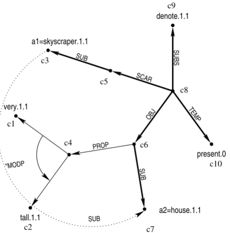
[image:3.595.180.410.70.303.2]a2=house.1.1 a1=skyscraper.1.1
Figure 1: Matching a pattern to an SN. Bold lines indicate matched arcs, the dashed line the inferred arc.
The SNs as described here are automati-cally constructed from (German) texts by the deep linguistic parser WOCADI3(Hartrumpf,
2002) whose parsing process is based on a word class functional analysis.
4 Application of Deep Patterns
The extraction of hyponyms as described here is based on a set of patterns. Each pattern consists of a conclusion partsub0(a1,a2) and a premise part in form of an SN where botha1
anda2 have to show up. The patterns are ap-plied by a pattern matcher (or automated the-orem prover if axioms are used) which matches the premise with an SN. The variable bindings fora1 and a2 are given by the matched con-cepts of the SN. An example pattern which matches to the sentence: A skyscraper de-notes a very tall building. is D4 (see
Ta-ble 1). The pattern matching process is il-lustrated in Fig.1. The resulting instantiated conclusion which is stored in the knowledge base is sub0(skyscraper.1.1, house.1.1). Ad-vantages by using the MultiNet SN formalism
3WOCADI is the abbreviation for word class
disambiguation.
for hypernym (and instance-of relation) acqui-sition consists of: learning relations between word readings instead of words, the possibil-ity to apply logical axioms and background knowledge, and that person names are already parsed.
An example sentence from the Wikipedia corpus where a hypernymy relation was suc-cessfully extracted by our deep approach and which illustrates the usefulness of this ap-proach is: In any case, not all incidents from the Bermuda Triangle or from other world areas are fully explained. From this sen-tence, a hypernymy pair cannot be extracted by the Hearst pattern X or other Y. The ap-plication of this pattern fails due to the word
from which cannot be matched. To extract this relation by means of shallow patterns an additional pattern would have to be intro-duced. This could also be the case if syntactic patterns were used instead since the coordina-tion of Bermuda Triangle and world areas is not represented in the syntactic constituency tree but only on a semantic level4.
4Note that some dependency parsers normalize
5 Graph Substructure Learning By Following the Minimum
Description Length Principle
In this section, we describe how the patterns can be learned by a supervised machine learn-ing approach followlearn-ing the Minimum Descrip-tion Length principle. This principle states that the best hypothesis for a given data set is that one which minimizes the description of the data (Rissanen, 1989), i.e., compresses the data the most. Basically we follow the substructure learning approach of Cook and Holder (Cook and Holder, 1994).
According to this approach, the description length to minimize is the number of bits re-quired to encode a certain graph which is com-pressed by means of a substructure. If a lot of graph vertices can be matched with the substructure vertices, this description length will be quite small. For our learning scenario we investigate collection of SNs containing a known hypernymy relationship. A pattern (given by a substructure in the premise) which compresses this set quite well is expected to be useful for extracting hypernyms.
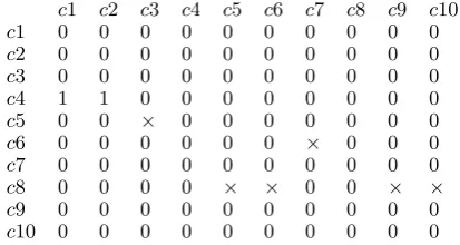
Let us first determine the number of bits to encode the entire graph or SN. A graph can be represented by its adjacency matrix and a set of vertex and arc labels. Since an adjacency matrix consists only of ones and zeros, it is well suitable for a binary encoding. For the encoding process, we do not regard the label names directly but instead their number as-suming an ordering exists on the label names (e.g., alphabetical).
c1 c2 c3 c4 c5 c6 c7 c8 c9 c10
c1 0 0 0 0 0 0 0 0 0 0
c2 0 0 0 0 0 0 0 0 0 0
c3 0 0 0 0 0 0 0 0 0 0
c4 1 1 0 0 0 0 0 0 0 0
c5 0 0 1 0 0 0 0 0 0 0
c6 0 0 0 0 0 0 1 0 0 0
c7 0 0 0 0 0 0 0 0 0 0
c8 0 0 0 0 1 1 0 0 1 1
c9 0 0 0 0 0 0 0 0 0 0
[image:4.595.79.278.582.691.2]c10 0 0 0 0 0 0 0 0 0 0
Figure 2: Adjacency matrix of the SN.
To encode all labels the number of labels and a list of all label numbers have to be spec-ified, e.g.,3,1,2,1 for 3 vertices with two dif-ferent label numbers5 (1,2). The first number encoding (3) starts at position 0 in the bit string, the second (1) at position 2 =dlog23e, the third one at position 2+dlog22e, etc. Since the graph actually need not to be encoded in this way but only the length of the encoding is important, non-integer numbers of bits are accepted for simplicity too. If there are a total of lu different labels, then each encoded label
number requires log2(lu) bits. The total
num-ber of bits to encode the vertex labels are then given by:
vbits= log2(v) +vlog2(lu) in whichvdenotes
the total number of vertices6.
In the next step, the adjacency matrix is en-coded where each row is processed separately. A straightforward approach for encoding one row would be to usev number of bits, one for every column. However, the number of zeros are generally much larger than the number of ones which means that a better compression of the data is possible by exploiting this fact. Consider the case that a certain matrix row contains exactly m ones. There are
v m
possibilities to distribute the ones to the indi-vidual cells. All possible permutations could be specified in a list. In this case it is only necessary to specify the position in this list to uniquely describe one row. Let b = maxiki.
Then the number of ones in one row can be encoded using log2(b+ 1) bits. log2
v ki
bits are required to encode the distribution of ones in one row. Additionally, log2(b+ 1) bits are needed to encodebwhich is only nec-essary once for the matrix. Let us consider the adjacency matrix given in Fig. 2 of the SN shown in Fig. 1 with 10 rows and columns where each row contains at most four ones. To encode the rowc4, containing two ones,
re-5The commas are only included for better
readabil-ity and are actually not encoded.
6The approach of Cook and Holder is a bit
quires log2(4) + log2
10 2
=7.49 bits which
is smaller than 10 bits which were necessary for the na¨ıve approach. The total lengthrbits
of the encoding is given by:
rbits= log2(b+ 1) +
v
X
i=1
[log2(b+ 1)+
log2
v ki
]
(1)
=(v+ 1) log2(b+ 1)+
v
X
i=1
log2
v ki
Finally, the arcs need to be encoded. Let e(i, j) be the number of arcs between vertex i and j in the graph and m := maxi,je(i, j).
log2(m) bits are required to encode the num-ber of arcs between both vertices and log2(le)
bits are needed for the arc label (out of a set of le elements). Then the entire number of
bits is given by (eis the number of arcs in the graph):
ebits= log2(m) +
v
X
i=1
v
X
j=1
[A[i, j]log2(m)+
e(i, j) log2(le)]
= log2(m) +elog2(le)+ v
X
i=1
v
X
j=1
A[i, j] log2(m)
=e(log2(le)) + (K+ 1) log2(m)
(2)
where K is the number of ones in the adja-cency matrix.
The total description length of the graph is then given by: vbits+rbits+ebits.
Now let us investigate how the description length of the compressed graph is determined. In the original algorithm the substructure is replaced in the graph by a single vertex. The description length of the graph compressed by the substructure is then given by the descrip-tion length of the substructure added by the description length of the modified graph.
c1 c2 c3 c4 c5 c6 c7 c8 c9 c10
c1 0 0 0 0 0 0 0 0 0 0
c2 0 0 0 0 0 0 0 0 0 0
c3 0 0 0 0 0 0 0 0 0 0
c4 1 1 0 0 0 0 0 0 0 0
c5 0 0 × 0 0 0 0 0 0 0
c6 0 0 0 0 0 0 × 0 0 0
c7 0 0 0 0 0 0 0 0 0 0
c8 0 0 0 0 × × 0 0 × ×
c9 0 0 0 0 0 0 0 0 0 0
[image:5.595.307.514.83.193.2]c10 0 0 0 0 0 0 0 0 0 0
Figure 3: Adjacency matrix of the compressed SN. Vertices whose connections can be com-pletely inferred from the pattern are removed.
In our method there are two major differ-ences from the graph learning approach of Cook and Holder.
• Not a single graph is compressed but a set of graphs.
• For the approach of Cook and Holder, it is unknown which vertex of the substruc-ture a graph node is actually connected with. Thus, the description is not com-plete and the original graph could not be reconstructed using the substructure and the compressed graph. To make the de-scription complete we specify the bind-ings of the substructure vertices to the graph vertices.
The generalization of the Cook and Holder-algorithm to a set of graphs is quite straight forward. The total description length of a set of compressed graphs is given by the descrip-tion length of the substructure (here pattern) added to the sum of the description lengths of each SN compressed by this pattern.
Additional bits are needed to encode the vertex bindings (assuming the pattern premise is contained in the SN). First the number of bindings bin ([1, vp], vp: number of
non-lexicalized vertices appearing in a pattern) has to be specified which requires log2(vp) bits.
The number of bits needed to encode a single binding is given by log2(vp) + log2(v) (vertex
number of required bits is given by
binbits =bin(log2(vp) + log2(v))+
log2(vp)
(3)
Note that not all bindings need to be coded. The number of required binding en-codings can be determined as follows. First all bindings for all non-lexicalized pattern ver-tices are determined. Then all cells from the adjacency matrix of the SN which contain a one and are also contained in the adjacency matrix of the pattern, if this binding is ap-plied to the non-lexicalized pattern vertices, are set to zero. Vertices which contain only ze-ros in the adjacency matrix on both columns and rows are removed from the adjacency ma-trix/graph. The arcs from and to this ver-tex can be completely inferred by the pattern which means that all vertices this vertex is connected with are also contained in the pat-tern. Since SNs differing only by the IDs of their non-lexicalized vertices are considered identical, no binding has to be specified for such a vertex. Additionally, the modified ad-jacency matrix is the result of the compres-sion by the pattern, i.e., vbits, rbits, and ebits are determined from the modified adjacency matrix/graph if the pattern was successfully matched to the SN.
Let us consider our example pattern D4
(Table 1). The following bindings are deter-mined: a1: c3 (a1); a: c8; c: c6; b: c5; a2: c7 (a2)
The bindings for a1 and a2 need not to be remembered since all hyponym vertices are re-named to a1 and the hypernym vertices to
a2 in order to learn generic patterns for arbi-trary hypernyms/hyponyms. The cells of the adjacency matrix which are associated to the arcs: scar(c8,c5), sub(c5,a1), obj(c8,c6), subs(c8,c9), temp(c8, c10) are set to zero (marked by a cross in Fig. 3) since these arcs are also represented in the pattern using the bindings stated above. The rows and columns of c3, c5, c7, and c9 of the modified graph adjacency matrix only contain zeros. Thus, these rows can be removed from the adja-cency matrix and the associated concepts can
be eliminated from the vertex set of the SN. The findings of the optimal patterns is done compositionally employing a beam search ap-proach. First this approach starts with pat-terns containing only a single arc. These patterns are then extended by adding one arc after another preferring patterns lead-ing to small description lengths of the com-pressed SNs. Note that only pattern premises are allowed which are fully connected, e.g., sub(a, c)∧sub(e, f) is no acceptable premise. Two lists are used during the search,
local besti for guiding the search process and
global best for storing the best global results found so far:
• local besti: The k best patterns of
lengthi
• global best: The k best patterns of any length
The list local besti is determined by
extend-ing all elements from local besti−1 by one
arc and only keeping the k arcs leading to the smallest description length. The list global best is updated after each change of the list local besti. This process is iterated
as long as the total description length can be further reduced, i.e., DL(local besti+1[0]) <
DL(local besti[0]), where DL :Pattern → R
denotes the description length of a pattern and [0] accesses the first element of a list.
The listglobal best contains as the result of this approach thekpatterns with the smallest overall compressed description length7. Note however that it is often not recommended to use all elements of global best since this list contains oftentimes patterns where the premise part is a subgraph (can be inferred by) another premise pattern part contained in this list and their combination would actually not reduce the description length. Thus, in addition to the original approach of Cook and Holder, a dependency resolution is done.
The following iterative approach is pro-posed to cancel out such dependent patterns: 1. Start with the first entry of the global list:
depend best :={global best[0]}
7compressed description length: short for
ID Definition Matching Expression
D1
sub0(a1,a2)←
sub(g,a2)∧attch(g, f)∧
subr(e,sub.0)∧temp(e,present.0)∧
arg2(e, f)∧arg1(e, d)∧
sub(d,a1)
An applehypo is a type
of fruithyper.
D2
sub0(a1,a2)←
sub(f,a2)∧equ(g, f)∧
subr(e,equ.0)∧temp(e,present.0)∧
arg2(e, f)∧arg1(e, d)∧
sub(d,a1)
Psycho-linguisticshypo is a sciencehyper
of the human ability to speak.
D3
sub0(a1,a2)←
pred(g,a2)∧attch(g, f)∧
subr(e,pred.0)∧arg2(e, f)∧
temp(e,present.0)∧arg1(e, d)∧
pred(d,a1)
Hepialidaehypo are a kind of insectshyper.
literal translation from: Die Wurzelbohrer sind eine Familie der Schmetterlinge.
D4
sub0(a1,a2)←
sub(f,a2)∧subs(e,denote.1.1)∧
temp(e,present.0)∧obj(e, f)∧
scar(e, d)∧sub(d,a1)
A skyscraperhypo
denotes a very tall buildinghyper.
D5
sub0(a1,a2)←
prop(f,other.1.1)∧pred(f,a2)∧
foll*itms(d, f)∧pred(d,a1)
duckshypo and other
animalshyper
D6 sub0sub(d,(a1a2,)a2)←
∧sub(d,a1) the instrumenthyper cellohypo
D7
sub0(a1, a2)←sub(f,a2)∧
temp(e,present.0)∧subr(e,sub.0)∧
sub(d,a1)∧arg2(e, f)∧
arg1(e, d)
The Morton numberhypois a
[image:7.595.74.457.68.366.2]dimensionless indicatorhyper.
Table 1: A selection of automatically learned patterns.
2. Setindex:=1
3. Calculate the combined (compressed) description length of depend best and
{global best[index]}
4. If the combined description length is reduced add global best[index] to
depend best, otherwise leavedepend best
unchanged
5. If counter ≥length(global best) then re-turndepend best
6. index :=index+ 1 7. Go back to step 3
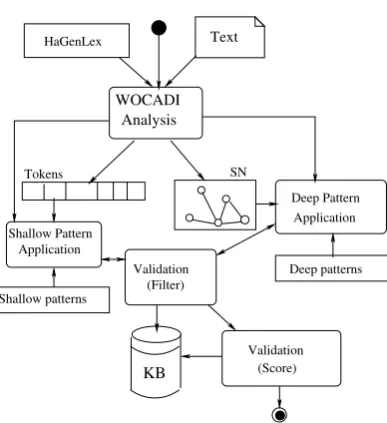
6 System Architecture
In this section, we give an overview over our hypernymy extraction system. The following procedure is employed to identify hypernymy relations in Wikipedia (see Fig. 4):
1. At first, all sentences of Wikipedia are analyzed by the deep analyzer WOCADI (Hartrumpf, 2002). As a result of the parsing process, a token list, a syntactic dependency tree, and an SN is created.
Tokens SN
Shallow Pattern Application
Shallow patterns
Deep patterns HaGenLex Text
Deep Pattern Application
Validation (Filter)
Validation (Score)
Analysis WOCADI
KB
[image:7.595.315.509.434.646.2]2. Shallow patterns based on regular expres-sions are applied to the token lists, and deep patterns (learned and hand-crafted) are applied to the SNs to generate pro-posals for hypernymy relations.
3. A validation tool using ontological sorts and semantic features checks whether the proposals are technically admissible at all to reduce the amount of data to be stored in the knowledge base KB.
4. If the validation is successful, the hyper-nymy hypothesis is integrated into KB. Steps 2–4 are repeated until all sentences are processed.
5. Each hypernymy hypothesis in KB is as-signed a confidence score estimating its reliability.
7 Validation Features
The knowledge acquisition carried out is fol-lowed by a two-step validation. In the first step, we check the ontological sorts and se-mantic features of relational arguments for subsumption. For instance, a discrete con-cept (ontological sort: d) denoting a human being (semantic feature: human +) can only be hypernym of an other object, if this object is both discrete and a human being as well. Only relational candidates for which semantic features and ontological sorts can be shown to be compatible are stored in the knowledge base.
In a second step, each relational candidate in the knowledge base is assigned a quality score. This is done by means of a support vector machine (SVM) on several features. The SVM determines the classification (hy-pernymy or non-hy(hy-pernymy) and a probabil-ity value for each hypernymy hypothesis. If the classification is ’hypernymy’, the score is defined by this probability value, otherwise as one minus this value.
Correctness Rate: The feature Correctness Rate takes into account that the assumed hy-pernym alone is already a strong indication for the correctness or incorrectness of the in-vestigated relation. The same holds for the assumed hyponym as well. For instance,
re-lation hypotheses with hypernym liquid and
town are usually correct. However, this is not the case for abstract concepts. Moreover, movie names are often extracted incompletely since they can consist of several tokens. Thus, this indicator determines how often a concept pair is classified correctly if a certain concept shows up in the first (hyponym) or second (hy-pernym) position.
Frequency: The feature frequency regards the quotient of the occurrences of the ponym in other extracted relations in hy-ponym position and the hypernym in hyper-nym position.
This feature is based on two assumption. First, we assume that general terms normally occur more frequently in large text corpora than very specific ones (Joho and Sanderson, 2007). Second, we assume that usually a hy-pernym has more hyponyms than vice-versa.
Context: Generally, the hyponym can ap-pear in the same textual context as its hyper-nym. The textual context can be described as a set of other concepts (or words for shallow approaches) which occur in the neighborhood of the investigated hyponym/hypernym can-didate pair investigated on a large text cor-pus. Instead of the textual context we re-gard the semantic context. More specifically, the distributions of all concepts are regarded which are connected with the assumed hyper-nym/hyponym concept by the MultiNet-prop (property) relation. The formula to estimate the similarity was basically taken from (Cimi-ano and others, 2005).
ID Precision First Sent. # Matches
D1 0.275 0.323 5 484
D2 0.183 0.230 35 497
D3 0.514 0.780 937
D4 0.536 0.706 1 581
D5 0.592 - 3 461
[image:8.595.308.516.558.654.2]D6 0.171 0.167 37 655
Table 2: Precision of hypernymy hypotheses extracted by patterns without usage of the val-idation component (D7 not yet evaluated).
de-Score ≥0.95 ≥0.90 ≥0.85 ≥0.80 ≥0.75 ≥0.70 ≥0.65 ≥0.60 ≥0.55 Precision 1.0000 0.8723 0.8649 0.8248 0.8203 0.7049 0.6781 0.5741 0.5703
Table 3: Precision of the extracted hypernymy relations for different confidence score intervals.
tailed description of the validation features.
8 Evaluation
We applied the pattern learning process on a collection of 600 SN, derived by WOCADI from Wikipedia, which contain hyponymically related concepts. Table 1 contains some of the extracted patterns including a typical expres-sion to which this pattern could be matched. The predicate f ollf(a, b) used in this table
specifies that argument a precedes argument b in the argument list of functionf. Patterns D1-D4 and D7 contain concept definitions
where the defined concept is, in many cases, the hyponym of the defining concept. In pat-ternD1andD7the defining concept is directly
identified by the parser as hypernym of the de-fined concept (subr(e,sub.0)). In patternD2
the defining concept is recognized as equiva-lent to the defined concept (subr(e,equ.0)). However, in most of the cases the defining concept consists of a meaning molecule, i.e., a complex concept where some inner concept is modified by an additional expression (often a property or an additional subclause). If this expression is dropped which is done by the pattern D2 the remaining concept becomes a
hypernym of the defined concept. Pattern D5
is a well-known Hearst pattern. Pattern D6
is used to match to appositions. However, for that the representation of appositions in the SN, as provided by the parser, could be im-proved since the order of the two concepts in a sentence is not clear by regarding only the SN, i.e., from the expression the instrument cello both sub0(instrument.1.1,cello.1.1) and sub0(cello.1.1,instrument.1.1) could be extracted. The incorrect relation hypoth-esis has to be filtered out (hopefully) by the validation component. A bet-ter representation would be by employ-ing the tupl*(c1, . . . , cn) predicate which
combines several concepts with regard to
their order. So the example expression should better be represented by sub(d, e) ∧
tupl*(e,instrument.1.1,cello.1.1).
Precision values for the hyponymy relation hypotheses extracted by the learned patterns, which are applied on a subset of the German Wikipedia, are given in Table 2. The first precision value specifies the overall precision, the second the precision if only hypernymy hy-potheses are considered which were extracted from first sentences of Wikipedia articles. The precision is usually increased considerably if only such sentences are regarded. Note that this precision value was not given for pattern D5 which usually cannot be matched to such
sentences. The last number specifies the to-tal amount of sentences a pattern could be matched to.
Furthermore, besides the pattern extraction process, the entire hypernymy acquisition sys-tem was validated, too. In total 391 153 dif-ferent hypernymy hypotheses were extracted employing 22 deep and 19 shallow patterns. 149 900 of the relations were only determined by the deep but not by the shallow patterns which shows that the recall can be consider-ably increased by using deep patterns in addi-tion. But also precision profits from the usage of deep patterns. The average precision of all relations extracted by both shallow and deep patterns is 0.514 that is considerably higher than the average precision for the relations only extracted by shallow patterns (0.243).
The correctness of an extracted relation hy-pothesis is given for several confidence score intervals in Table 3. There are 89 944 con-cept pairs with a score above 0.7, 3 558 of them were annotated with the information of whether the hypernymy relation actually holds.
from a text corpus has to be known where different annotators can have very dissenting opinions about this number. Thus, we just gave the number of relation hypotheses ex-ceeding a certain score. However the precision obtained by our system is quite competitive to other approaches for hypernymy extrac-tion like the one of Erik Tjong and Kim Sang which extracts hypernyms in Dutch (Tjong and Sang, 2007) (Precision: 0.48).
9 Conclusion and Outlook
We showed a method to automatically derive patterns for hypernymy extraction in form of SNs by following the MDL principle. A list of such patterns together with precision and number of matches were given to show the usefulness of the applied approach. The pat-terns were applied on the Wikipedia corpus to extract hypernymy hypotheses. These hy-potheses were validated using several features. Depending on the score, an arbitrary high pre-cision can be reached. Currently, we deter-mine confidence values for the precision values of the pattern example. Further future work includes the application of our learning algo-rithm to larger text corpora in order to find additional patterns. Also an investigation of how this method can be used for other types of semantic relations is of interest.
Acknowledgements
We want to thank all of our department which contributed to this work, especially Sven Hartrumpf and Alexander Pilz-Lansley for proofreading this paper. This work was in part funded by the DFG project Semantis-che Duplikatserkennung mithilfe von Textual Entailment (HE 2847/11-1).
References
Cimiano, P. et al. 2005. Learning taxonomic re-lations from heterogeneous sources of evidence. In Buitelaar, P. et al., editors, Ontology Learn-ing from Text: Methods, evaluation and applica-tions, pages 59–73. IOS Press, Amsterdam, The Netherlands.
Cook, D. and L. Holder. 1994. Substructure dis-covery using minimum description length and background knowledge. Journal of Artificial In-telligence Research, 1:231–255.
Fellbaum, C., editor. 1998. WordNet An Elec-tronic Lexical Database. MIT Press, Cam-bridge, Massachusetts.
Hamp, B. and H. Feldweg. 1997. Germanet - a lexical-semantic net for german. InProc. of the ACL workshop of Automatic Information Ex-traction and Building of Lexical Semantic Re-sources for NLP Applications, Madrid, Spain.
Hartrumpf, S. et al. 2003. The semantically based computer lexicon HaGenLex – Structure and technological environment. Traitement automa-tique des langues, 44(2):81–105.
Hartrumpf, S. 2002. Hybrid Disambiguation in Natural Language Analysis. Ph.D. thesis, Fern-Universit¨at in Hagen, Fachbereich Informatik, Hagen, Germany.
Hearst, M. 1992. Automatic acquisition of hy-ponyms from large text corpora. In Proc. of COLING, Nantes, France.
Helbig, H. 2006. Knowledge Representation and the Semantics of Natural Language. Springer, Berlin, Germany.
Joho, H. and M. Sanderson. 2007. Document fre-quency and term specificity. InProc. of RIAO, Pittsburgh, Pennsylvania.
Morin, E. and C. Jaquemin. 2004. Automatic acquisition and expansion of hypernym links.
Computers and the Humanities, 38(4):363–396.
Rissanen, J. 1989. Stochastic Complexity in Statistical Inquiry. World Scientific Publishing Company, Hackensack, New Jersey.
Snow, R. et al. 2005. Learning syntactic patterns for automatic hypernym discovery. InAdvances in Neural Information Processing Systems 17, pages 1297–1304. MIT Press, Cambridge, Mas-sachusetts.
Tjong, E. and K. Sang. 2007. Extracting hy-pernym pairs from the web. In Proceedings of the 45 Annual Meeting of the ACL on In-teractive Poster and Demonstration Sessions, Prague, Czech Republic.