Engineering Statistical Dialog State Trackers: A Case Study on DSTC

(1)

Engineering Statistical Dialog State Trackers: A Case Study on DSTC

Daejoong Kim, Jaedeug Choi, Kee-Eung Kim Department of Computer Science, KAIST

South Korea

{djkim, jdchoi, kekim}@ai.kaist.ac.kr

Jungsu Lee, Jinho Sohn LG Electronics

South Korea

{jungsu.lee, jinho.sohn}@lge.com

Abstract

We describe our experience with engineer-ing the dialog state tracker for the first Dialog State Tracking Challenge (DSTC). Dialog trackers are one of the essential components of dialog systems which are used to infer the true user goal from the speech processing results. We explain the main parts of our tracker: the observation model, the belief refinement model, and the belief transformation model. We also report experimental results on a number of approaches to the models, and compare the overall performance of our tracker to other submitted trackers. An extended ver-sion of this paper is available as a technical report (Kim et al., 2013).

1 Introduction

In spoken dialog systems (SDSs), one of the main challenges is to identify the user goal from her ut-terances. The significance of accurately identify-ing the user goal, referred to as dialog state track-ing, has emerged from the need for SDSs to be robust to inevitable errors in the spoken language understanding (SLU).

A number of studies have been conducted to track the dialog state through multiple dialog turns using a probabilistic framework, treating SLU re-sults as noisy observations and maintaining prob-ability distribution (i.e., belief) on user goals (Bo-hus and Rudnicky, 2006; Mehta et al., 2010; Roy et al., 2000; Williams and Young, 2007; Thomson and Young, 2010; Kim et al., 2011).

In this paper, we share our experience and lessons learned from developing the dialog state tracker that participated in the first Dialog State Tracking Challenge (DSTC) (Williams et al., 2013). Our tracker is based on the belief up-date in the POMDP framework (Kaelbling et al.,

1998), particularly the hidden information state (HIS) model (Young et al., 2010) and the partition recombination method (Williams, 2010).

2 Dialog State Tracking

Our tracker mainly follows the belief update in HIS-POMDP (Young et al., 2010). The SDS ex-ecutes system action a, and the user with goal

g responds to the system with utterance u. The SLU processes the utterance and generates the re-sult as anN-best listo= [_hu˜1, f1i, . . . ,hu˜N, fNi] of the hypothesized user utterance u˜i and its as-sociated confidence score fi. Because the SLU is not perfect, the system maintains a probability distribution over user goals, called a belief. In ad-dition, the system groups user goals into equiva-lence classes and assigns a single probability for each equivalence class since the number of user goals is often too large to perform individual be-lief updates for all possible user goals. The equiv-alence classes are called partitions and denoted as

ψ. Hence, given the current beliefb, system action

a, and recognizedN-best list o, the dialog state tracker updates the beliefb′over partitions as fol-lows:

b′(ψ′)_∝X

u

Pr(o_|u) Pr(u_|ψ′, a) Pr(ψ′_|ψ)b(ψ)

(1) where Pr(o_|u) is the observation model,

Pr(u_|ψ, a) is the user utterance model,Pr(ψ′_|ψ)

is the belief refinement model.

2.1 Observation Model

The observation modelPr(o_|u)is the probability that the SLU produces theN-best listowhen the user utterance isu. We experimented with the fol-lowing three models for the observation model.

Confidence score model: as in HIS-POMDP,

this model assumes that the confidence score fi obtained from the SLU is exactly the probability

(2)

of generating the hypothesized user utterance u˜i. Hence,fi = Pr(˜ui, fi|u).

Histogram model: this model estimates a

func-tion that maps the confidence score to the proba-bility of correctness. We constructed a histogram of confidence scores from the training datasets to obtain the empirical probabilityPr(cor(fi))of whether the entry associated with confidence score

fiis a correct hypothesis or not.

Generative model: this model is a simplified

version of a generative model in (Williams, 2008) that only uses confidence score: Pr(˜ui, fi|u) =

Pr(cor(i)) Pr(fi|cor(i))wherePr(cor(i))is the probability of the i-th entry being a correct hy-pothesis andPr(fi|cor(i))is the probability of the

i-th entry having confidence scorefi when it is a correct hypothesis.

2.2 User Utterance Model

The user utterance model Pr(u_|ψ, a) indicates how the user responds to the system action a

when the user goal is in ψ. We adopted the HIS-POMDP user utterance model, consisting of a bi-gram model and an item model. The details are described in (Kim et al., 2013).

2.3 Belief Refinement Model

Given the SLU result u˜i and the system action

a, the partition ψ is split into ψ′_i with probabil-ityPr(ψ_i′|ψ)andψ−ψ_i′ with probabilityPr(ψ−

ψ′_i|ψ). The belief refinement modelPr(ψ_i′|ψ)can be seen as the proportion of the belief that is car-ried fromψtoψ′

i. This probability can be defined by the following models:

Empirical model: we count n(ψ) from the training datasets, which is the number of user goals that are consistent with partition ψ. The probability is then modeled asPr(ψ′_i_|ψ) = n(ψi′)

n(ψ)

ifn(ψ)>0andPr(ψ_i′_|ψ) = 0otherwise.

Word-match model: this model extends the

empirical model by using the domain knowledge when the SLU result u˜i does not appear in the training datasets. We calculated how many words

w ∈ W in the user utteranceu˜i were included in a bus timetableD. The model is thus defined as

Pr(ψ′_i_|ψ) = n(ψ′i)

n(ψ) ifn(ψi′) > 0andPr(ψi′|ψ) = α

|W| P

w∈W δ(w ∈ D)otherwise. δis the indica-tor function (δ(x) = 1 if x holds andδ(x) = 0

otherwise) and α is the parameter estimated via cross-validation.

Mixture model: this model mixes the

empiri-cal model with a uniform probability, defined as

Pr(ψ′_i|ψ) =ǫ_n1

G + (1−ǫ)

n(ψ′

i)

n(ψ) ifn(ψi′)>0and

Pr(ψ′_i_|ψ) = _n1

G otherwise.nGis the number of all

possible user goals which is treated as the param-eter of the model and found via cross-validation, together with the mixing parameterǫ_∈[0,1].

2.4 Belief Transformation Model

The belief update described above pro-duces the M-best hypotheses of user goals

[_hg˜1, b(˜g1)i, . . . ,hg˜M, b(˜gM)i]in each dialog turn, which consists of M most likely user goal hy-potheses˜giand their associated beliefsb(˜gi). The last hypothesisg˜M is reserved as the null hypoth-esis∅with the belief b(∅) = 1−PiM=1−1b(˜gi), which represents that the user goal is not known up to the current dialog turn.

One of the problems with the belief update is that the null hypothesis often remains as the most probable hypothesis even when the SLU result contains the correct user utterance with a high con-fidence score. This is because an atomic hypothe-sis has a very small prior probability.

To overcome this problem, we added a post-processing step which transforms each beliefb(hi) to the final confidence scoresi.

Threshold model: this model ensures that the

top hypothesis has confidence scoreθwhen a be-lief of the hypothesis is greater than a thresholdδ. The final output list is[hh∗, s∗i,h∅,1−s∗i]where

h∗= argmax_h_∈{_˜_g1,...,_˜_g_M₋₁_}b(h)and

s∗ = (

θ, ifb(h∗)> δ

b(h∗), otherwise. (2)

Full-list regression model: this model

esti-mates the probability that each hypothesis is cor-rect via casting the task as regression. The model uses two logistic regression functions F_∅

and Fh. F∅ predicts the probability of correct-ness for the null hypothesis ∅ using the sin-gle input feature φ_∅ = b(∅). Likewise, Fh predicts the probability of correctness for non-null hypotheses hi using the input feature φi =

b(hi). The model generates the final output list [hh1, s1i, . . . ,hhM−1, sM−1i,h∅, sMi]where

hi= ˜giand

si =

  

F_∅(φi) PM−1

j=1 Fh(φj)+F∅(φ∅), ifi=M

Fh(φi) PM−1

j=1 Fh(φj)+F∅(φ∅), otherwise.

(3)

Rank regression model: this model works in

a similar way as in the full-link regression model, except that it uses a single logistic regression func-tion Fr for both the non-null and null hypothe-ses, and takes the rank value of the hypotheses as an additional input feature. The final out-put list is [_hh1, s1i, . . . ,hhM−1, sM−1i,h∅, sMi] wherehi= ˜gi and

si= PMFr(φi)

j=1Fr(φj). (4)

3 Experimental Setup

In the experiments, we used three labeled train-ing datasets (train1a, train2, train3) and three test datasets (test1, test2, test3) used in DSTC. There was an additional test dataset (test4), which we decided not to include in the experiments since we found that a significant number of labels were missing or incorrect.

We measured the tracker performance accord-ing to the followaccord-ing evaluation metrics used in DSTC1: accuracy (acc) measures the rate of the most likely hypothesis h1 being correct, average score (avgp) measures the average of scores

as-signed to the correct hypotheses, l2 norm mea-sures the Euclidean distance between the vector of scores from the tracker and the binary vector with 1 in the position of the correct hypotheses, and 0 elsewhere, mean reciprocal rank (mrr) measures the average of 1/R, where R is the minimum rank of the correct hypothesis, ROC

equal error rate (eer) is the sum of false accept

(FA) and false reject (FR) rates when FA rate=FR rate, and ROC.{v1,v2}.Pmeasures correct accept (CA) rate when there are at mostP% false accept (FA) rate2.

4 Results and Analyses

Since there are multiple slots to track in the dialog domain, we report the average performance over the “marginal” slots including the “joint” slot that assigns the values to all slots.

4.1 Observation Model

Tbl. 1 shows the cross-validation results of the three observation models. In train1a and train2, no model had a clear advantage to others, whereas in

1

http://research.microsoft.com/apps/pubs/?id=169024 2_{There are two types of ROC measured in DSTC}

[image:3.595.307.535.72.225.2]

depend-ing on how CA and FA rates are calculated. The detailed dis-cussion is provided in the longer version of the paper (Kim et al., 2013).

Table 1: Evaluation of observation models.

Train1a Train2 Train3

Conf Hist Gen Conf Hist Gen Conf Hist Gen

accuracy 0.81 0.82 0.82 0.84 0.86 0.85 0.90 0.89 0.88 avgp 0.77 0.78 0.78 0.81 0.82 0.82 0.81 0.79 0.77 l2 0.31 0.30 0.30 0.26 0.25 0.25 0.25 0.27 0.30 mrr 0.87 0.87 0.88 0.89 0.89 0.89 0.94 0.93 0.92 roc.v1.05 0.69 0.70 0.70 0.73 0.74 0.74 0.82 0.80 0.79 roc.v1.10 0.74 0.75 0.75 0.78 0.80 0.80 0.87 0.85 0.83 roc.v1.20 0.78 0.79 0.79 0.83 0.84 0.84 0.89 0.87 0.85 roc.v1.eer 0.14 0.14 0.14 0.12 0.13 0.13 0.10 0.11 0.12 roc.v2.05 0.34 0.34 0.34 0.24 0.15 0.23 0.52 0.54 0.52 roc.v2.10 0.54 0.46 0.46 0.33 0.26 0.25 0.71 0.67 0.70 roc.v2.20 0.70 0.70 0.69 0.43 0.41 0.41 0.83 0.78 0.80

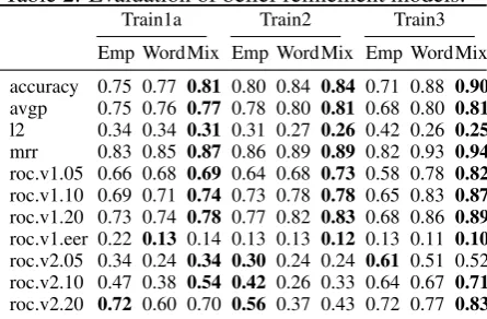
Table 2: Evaluation of belief refinement models.

Emp WordMix Emp WordMix Emp WordMix

train3, the confidence score model outperformed others. Further analyses revealed that the confi-dence scores from the SLU results were not suf-ficiently indicative of the SLU accuracy in train1a and train2. The histogram and the generative mod-els are expected to perform at least as well as the confidence score model in train3, but they didn’t in the experiments. We suspect that this is due to the naive binning strategy we used to model the probability distribution.

4.2 Belief Refinement Model

As shown in Tbl. 2, the mixture model outper-formed others throughout the metrics. It even outperforms the word-match model which tries to leverage the domain knowledge to handle novel user goals. This implies that, unless the domain knowledge is used properly, simply taking the mixture with the uniform distribution yields a suf-ficient level of performance.

4.3 Belief Transformation Model

[image:3.595.309.532.257.403.2]

(4)

Table 3: Evaluation of belief transform models.

Thre Full Rank Thre Full Rank Thre Full Rank

in the table. The full-list and the rank regres-sion models show a similar level of performance improvement. This is a naturally expected result since they use regression to convert the beliefs to final confidence scores, as an attempt to compen-sate for the errors incurred by approximations and assumptions made in the observation and belief re-finement models.

4.4 DSTC Result

In order to compare our tracker with others par-ticipated in DSTC, we chose tracker43as the most effective one among our 5 submitted trackers since it achieved the top scores in the largest num-ber of evaluation metrics. In the same way, we selected tracker2 for team3, tracker3 for team6, tracker3 for team8, and tracker1 for the rest of the teams. The results of each team are presented in Tbl. 4. The baseline tracker is included as a ref-erence, which simply outputs the hypothesis with the largest SLU confidence score in the N-best list.

Compared to other teams, our tracker showed strong performance in acc, avgp, l2 and mrr. A detailed discussion on the results is provided in the longer version of the paper (Kim et al., 2013).

5 Conclusion

In this paper, we described our experience with engineering a statistical dialog state tracker while participating in DSTC. Our engineering effort was focused on improving three important models in the tracker: the observation, the belief refine-ment, and the belief transformation models. Us-ing standard statistical techniques, we were able

3_{The tracker4 used the confidence score model, the}

mix-ture model and the rank regression model.

Table 4: Results of the trackers. The bold face denotes top 3 scores in each evaluation metric. T9 is our tracker.

Base T1 T2 T3 T4 T5 T6 T7 T8 T9

Test 1

accuracy 0.71 0.83 0.81 0.81 0.74 0.80 0.87 0.78 0.51 0.82 avgp 0.73 0.77 0.77 0.81 0.74 0.79 0.82 0.76 0.49 0.79 l2 0.38 0.32 0.32 0.27 0.37 0.30 0.25 0.34 0.72 0.29 mrr 0.80 0.88 0.86 0.85 0.81 0.85 0.90 0.84 0.59 0.88 roc.v1.05 0.62 0.72 0.67 0.60 0.20 0.71 0.76 0.65 0.20 0.72 roc.v1.10 0.63 0.78 0.75 0.77 0.29 0.75 0.82 0.70 0.33 0.76 roc.v1.20 0.67 0.82 0.79 0.79 0.53 0.78 0.85 0.76 0.35 0.79 roc.v1.eer 0.24 0.13 0.25 0.24 0.74 0.12 0.12 0.15 0.52 0.14 roc.v2.05 0.49 0.64 0.01 0.02 0.00 0.55 0.16 0.19 0.04 0.26 roc.v2.10 0.69 0.71 0.14 0.03 0.00 0.68 0.39 0.35 0.05 0.47 roc.v2.20 0.71 0.80 0.48 0.29 0.00 0.74 0.59 0.58 0.27 0.62

Test 2

Test 3

to produce a tracker that performed competitively among the participants.

As for the future work, we plan to refine the user utterance model for improving the perfor-mance of the tracker since there are a number of user utterances that are not handled by the cur-rent model. We also plan to re-evaluate our tracker with properly handling the joint slot, since the cur-rent tracker constructs models independently for each marginal slot and then combines the results by simply multiplying the predicted scores.

Acknowledgement

(5)

References

Dan Bohus and Alex Rudnicky. 2006. A ”k hypothe-ses + other” belief updating model. In Proceedings

of the AAAI Workshop on Statistical and Empirical Approaches for Spoken Dialogue Systems.

Leslie Pack Kaelbling, Michael L. Littman, and An-thony R. Cassandra. 1998. Planning and acting in partially observable stochastic domains. Artificial

Intelligence, 101(1–2):99–134.

Dongho Kim, Jin Hyung Kim, and Kee-Eung Kim. 2011. Robust performance evaluation of POMDP-based dialogue systems. IEEE Transactions on

Au-dio, Speech, and Language Processing, 19(4):1029– 1040.

Daejoong Kim, Jaedeug Choi, Kee-Eung Kim, Jungsu Lee, and Jinho Sohn. 2013. Engineering statistical dialog state trackers:a case study on DSTC. Techni-cal Report CS-TR-2013-379, Department of Com-puter Science, KAIST.

Neville Mehta, Rakesh Gupta, Antoine Raux, Deepak Ramachandran, and Stefan Krawczyk. 2010. Prob-abilistic ontology trees for belief tracking in dialog systems. In Proceedings of the 11th Annual

Meet-ing of the Special Interest Group on Discourse and Dialogue (SIGDIAL), pages 37–46.

Nicholas Roy, Joelle Pineau, and Sebastian Thrun. 2000. Spoken dialogue management using proba-bilistic reasoning. In Proceedings of the 38th

An-nual Meeting on Association for Computational Lin-guistics (ACL), pages 93–100.

Blaise Thomson and Steve Young. 2010. Bayesian update of dialogue state: A POMDP framework for

spoken dialogue systems. Computer Speech and

Language, 24(4):562–588.

Jason D. Williams and Steve Young. 2007. Partially observable Markov decision processes for spoken dialog systems. Computer Speech and Language, 21(2):393–422.

Jason Williams, Antoine Raux, Deepak Ramachan-dran, and Alan Black. 2013. The dialog state track-ing challenge. In Proceedtrack-ings of the 14th Annual

Meeting of the Special Interest Group on Discourse and Dialogue (SIGDIAL).

Jason D. Williams. 2008. Exploiting the ASR N-best by tracking multiple dialog state hypotheses. In

Pro-ceedings of the 9th Annual Conference of the In-ternational Speech Communication Association (IN-TERSPEECH), pages 191–194.

Jason D. Williams. 2010. Incremental partition re-combination for efficient tracking of multiple dia-log states. In Proceedings of the IEEE International

Conference on Acoustics Speech and Signal Pro-cessing (ICASSP), pages 5382–5385.

Steve Young, Milica Gaˇsi´c, Simon Keizer, Franc¸ois Mairesse, Jost Schatzmann, Blaise Thomson, and Kai Yu. 2010. The hidden information state model: A practical framework for POMDP-based spoken di-alogue management. Computer Speech and