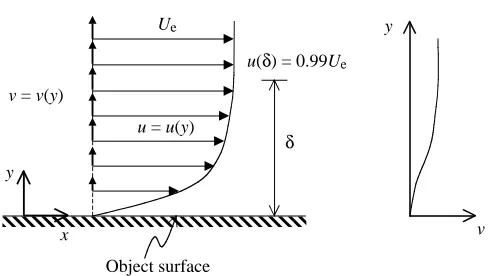
When a body moves relative to a surrounding fluid, a boundary layer exists very close to the body surface as a result of the ‘no-slip condition’ and viscosity (Prandtl, 1904). Consider an object held stationary in a uniform oncoming flow with velocity U. The fluid in direct contact with the body surface adheres to the surface and has zero velocity. The fluid just above the surface is slowed by frictional forces associated with the viscosity of the fluid. The closer the fluid is to the surface, the more it is slowed. The result is a thin layer where the tangential velocity, u, of the fluid increases from zero at the body surface to a velocity close to U. This velocity at the outer edge of the boundary layer, Ue, depends on the shape of the body (Schetz, 1993). By definition, the boundary layer extends from the object’s surface, y=0, to a position y=δ, where the tangential velocity relative to the object’s surface is 0.99Ue. The curve representing the continuous variation in tangential velocity from y=0 to y=δ is commonly referred to as the boundary layer profile or, more specifically, the u-profile
(Fig. 1). Normal velocity relative to the surface also varies from zero at the body surface to some external value, Ve, generating what is known as the v-profile (Fig. 1). A third profile, the w-profile, usually exists in the flow over three-dimensional surfaces, where w is tangential to the wall and perpendicular to u. Note that if u, v or w is not specified, the term ‘boundary layer profile’ generally refers to the u-profile. The shapes of the boundary layer profiles above a particular position on a surface depend on the shape of the body, surface roughness, the upstream history of the boundary layer, the surrounding flow field and Reynolds number. Flow in the boundary layer can be laminar or turbulent, resulting in radically different classes of profile shapes. Prandtl (1952), Schlichting (1979) and Batchelor (1967) provide thorough descriptions of the boundary layer concept. The behavior of a body moving relative to a real fluid cannot be accurately described without an understanding of the boundary layer. Since the work of Prandtl (1904), great strides have been made JEB2919
Tangential and normal velocity profiles of the boundary layer surrounding live swimming fish were determined by digital particle tracking velocimetry, DPTV. Two species were examined: the scup Stenotomus chrysops, a carangiform swimmer, and the smooth dogfish Mustelus
canis, an anguilliform swimmer. Measurements were taken
at several locations over the surfaces of the fish and throughout complete undulatory cycles of their propulsive motions. The Reynolds number based on length, Re, ranged from 3×10³ to 3×10⁵. In general, boundary layer profiles
were found to match known laminar and turbulent profiles including those of Blasius, Falkner and Skan and the law of the wall. In still water, boundary layer profile shape always suggested laminar flow. In flowing water, boundary layer profile shape suggested laminar flow at lower Reynolds numbers and turbulent flow at the highest Reynolds numbers. In some cases, oscillation between laminar and turbulent profile shapes with body phase was observed. Local friction coefficients, boundary layer thickness and fluid velocities at the edge of the boundary layer were suggestive of local oscillatory and mean
streamwise acceleration of the boundary layer. The behavior of these variables differed significantly in the boundary layer over a rigid fish. Total skin friction was determined. Swimming fish were found to experience greater friction drag than the same fish stretched straight in the flow. Nevertheless, the power necessary to overcome friction drag was determined to be within previous experimentally measured power outputs.
No separation of the boundary layer was observed around swimming fish, suggesting negligible form drag. Inflected boundary layers, suggestive of incipient separation, were observed sporadically, but appeared to be stabilized at later phases of the undulatory cycle. These phenomena may be evidence of hydrodynamic sensing and response towards the optimization of swimming performance.
Key words: undulatory swimming, fish, boundary layer, friction, drag, separation, hydrodynamics, digital particle image velocimetry, digital particle tracking velocimetry.
Summary
Introduction
THE BOUNDARY LAYER OF SWIMMING FISH
ERIK J. ANDERSON, WADE R. MCGILLIS ANDMARK A. GROSENBAUGH*
Department of Applied Ocean Physics and Engineering, Woods Hole Oceanographic Institution, Woods Hole, MA 02543, USA
*Author for correspondence (e-mail: mgrosenbaugh@whoi.edu)
in understanding fluid forces acting on bodies. Nevertheless, the hydrodynamics of undulatory swimming remains elusive. Drag, thrust and power in undulatory swimming have not been definitively determined. This is, in part, because no definitive measurements of boundary layer flow over a swimming fish or cetacean have been performed.
Few attempts have been made to characterize the boundary layers of undulatory swimmers, and none has produced boundary layer velocity profiles. Most recently, Rohr et al. (1998b) have suggested that the relative intensity of bioluminescence around a swimming dolphin may be linked to the thickness of the boundary layer. In a set of earlier investigations, Kent et al. (1961) and Allen (1961) achieved a qualitative description of flow in the near-field and possibly the boundary layers of fish using the Schlieren technique. The near-field is the region of flow around the fish affected by the presence of the fish and its swimming motions. In contrast, the so-called far-field is the region in which the impact of the fish has decayed essentially to nothing. While the boundary layer can certainly be considered part of the near-field flow, to aid in the discussion, we use the term near-field to refer to the region dominated by the presence of the fish, but outside the boundary layer.
The understanding of drag mechanisms in undulatory swimming has been impeded significantly by this lack of boundary layer data. Both form drag and friction drag on a
body depend on the nature of the boundary layer. Unlike the drag on a rigid body, such as an airplane wing, the drag on a swimming fish cannot be measured by simply placing a fish-shaped model in a wind or water tunnel. The boundary layer of a swimming fish is complicated by the motion of the body and is unquestionably different from that over a rigid model. Furthermore, since the drag- and thrust-producing mechanisms of a swimming fish are coupled, even the use of an actively swimming model requires indirect means to determine drag (Barrett et al., 1999). Gray (1936) was clearly skeptical of the extension of the so-called ‘rigid-body analogy’ to the determination of drag on a swimming dolphin but, left with no alternative, he used rigid-body drag as a tentative approximation. Webb (1975) catalogues the rigid-body drag calculations and measurements on fish that ensued, but reiterates the warning concerning the weakness of the analogy. The reservations of Gray (1936) were affirmed when Lighthill (1960, 1970, 1971) published his reactive model of fish propulsion, which predicted thrust in steady swimming to be as much as 3–5 times greater than the theoretical rigid-body drag. While the reactive thrust model of Lighthill (1960, 1970, 1971) is considered to overestimate thrust, it is widely believed that the drag on a swimming fish is, indeed, greater than rigid-body drag. Weihs (1974) determined that it was possible for fish to capitalize on this state of affairs by burst-and-coast swimming.
Lighthill (1971), citing discussions with Q. Bone, claims that this ‘enhanced friction drag’ may be the result of boundary layer effects resulting from the lateral movements of the body segments of swimming fish. The rate at which vorticity is produced as the body surface is thrust into the surrounding fluid is likely to be higher than the outward diffusion of vorticity that occurs during the retreat of the body surface. The result of this mechanism would be a boundary layer that is thinner and of higher shear than would be expected over the rigid body. Our fish boundary layer data substantiate this hypothesis and reveal an additional mechanism of friction drag enhancement – mean streamwise acceleration of the near-field flow.
Lighthill’s (1971) prediction of enhanced friction drag further confused the already troubled field of energetics in undulatory locomotion. Gray (1936) and Gero (1952), among others (Webb, 1975), made measurements that suggested that the power required to overcome rigid-body drag for dolphins and certain fish was greater than their muscle mass was capable of producing. This spawned a search for mechanisms that could reduce the drag on an undulatory swimmer to levels below the rigid-body drag. If, as Lighthill (1971) suggested, the drag on a swimming fish was actually several times the rigid-body drag, the situation became even more problematic. It was clear that Lighthill’s (1971) model over-predicted thrust, that swimming performances had been exaggerated or that the estimates of available muscle power were too low.
Investigators of undulatory swimming hydrodynamics and muscle physiology have studied each of these alternatives in an attempt to resolve the discrepancies. Thrust and power y
x
u = u(y) Ue
u(δ) = 0.99Ue
v = v(y)
y
v
Object surface
[image:2.612.46.294.66.204.2]δ
were estimated from velocity measurements of the wake of a swimming mullet Chelon labrosus (Müller et al., 1997). These investigators used techniques that were developed to calculate thrust and minimum muscle power output in bird and insect flight, where they were met with varied success (Rayner, 1979a,b; Ellington, 1984; Spedding et al., 1984; Spedding, 1986, 1987). In their preliminary work, Müller et al. (1997) report thrust estimates even higher than the theoretical values of Lighthill (1971). At the same time, claims of extraordinary performances of undulatory swimmers have been toned down somewhat (Lighthill, 1969; Rohr et al., 1998a) and estimates of available muscle power have been refined (Bainbridge, 1961; Webb, 1975; Weis-Fogh and Alexander, 1977; Fish, 1993; Rome et al., 1993; Coughlin et al., 1996). In the light of such findings, it appears less incumbent upon fish and cetaceans to possess extraordinary drag-reducing secrets (Fish and Hui, 1991). Still, the problem has not been unequivocally resolved. Excised fish muscle driven at rates equal to those measured in vivo has given relatively low power outputs (Rome and Swank, 1992; Coughlin et al., 1996; Swank and Rome, 2000; Rome et al., 2000). These studies suggest that maximum power output measurements recorded during non-physiological stimulation and strain are not applicable.
Despite the dearth of available boundary layer data and Lighthill’s (1971) prediction of drag enhancement based on theoretical thrust, theories of drag reduction by boundary layer manipulation abound. The most notable proposed mechanisms fall under the categories of laminar boundary layer maintenance, turbulent drag reduction, utilization of shed vorticity and the delay of separation. Theories of drag reduction in undulatory swimming are reviewed and critised in Webb (1975), Webb and Weihs (1983) and Fish and Hui (1991). One recent experimental study using a robotic fish claims to have substantiated drag reduction in undulatory swimming (Barrett et al., 1999). Earlier works, on the flow over waving plates, have also demonstrated mechanisms that may act to reduce drag, especially form drag. Taneda and Tomonari (1974) observed that the flow over a waving plate with wave speed c, less than the oncoming flume speed U, resulted in separation of flow and turbulent recirculation regions in the wave troughs. When wave speed was increased so that c/U⭓1, flow remained attached over the entire plate. In some cases, boundary layer flow was completely laminarized. In others, it oscillated between turbulent and laminar.
Here, we present the first description of boundary layer flow in swimming fish based on high-resolution velocity profiles. We report the unsteady spatial distribution of boundary-layer-related variables over the surface of swimming fish and discuss mechanisms responsible for the observed behaviors. The distribution of wall shear stress, determined from the boundary layer, is used to determine the total friction drag and the power necessary to overcome it. Theories of boundary layer manipulation, drag reduction and friction drag enhancement are re-examined.
Materials and methods Fish
Scup Stenotomus chrysops (N=9) and smooth dogfish Mustelus canis (N=1) were caught in traps or by hook and line in Nantucket Sound, off Woods Hole, MA, USA. The animals were kept in 750 l tanks with a constant flow of fresh sea water from Nantucket Sound. All fish kept longer than 2 days were fed frozen squid biweekly. Fish were transferred to and from their tanks in 30 l buckets or 60 l coolers. Following experiments, fish were killed by cervical transection. The body length, L, of scup averaged 19.5±1.8 cm (mean ± S.D.). The dogfish measured 44.4 cm.
Swimming conditions
Scup were observed swimming both in still water and in a flume. In still water, scup were observed swimming at 3–40 cm s−1 at water temperatures of 11 °C or 22–25 °C, depending on the season during which the experiments were run. In the flume, scup were observed swimming at 10–65 cm s−1 at 22–23 °C. The dogfish was observed swimming at 20–65 cm s−1in the flume at 22–23 °C.
In flume trials, observations from three positions along the midline of each fish were made at one or more speeds. In scup, the measurements were made at x=0.50L, 0.77L and 0.91L. In dogfish, the measurements were made at x=0.44L, 0.53L and 0.69L. The majority of flume data for scup were acquired at a swimming speed of 30 cm s−1 (18 swimming sequences). At this speed, scup were observed to use primarily caudal fin propulsion with infrequent strokes by their pectoral fins. Recordings of transverse velocity showed continuous undulatory swimming during all acquired sequences. In still water, scup tended to swim more slowly, frequently using their pectoral fins and gliding. Therefore, in our analysis of the fish boundary layer, we have concentrated on the flume experiments and the fastest of the still-water swimming sequences. The majority of the flume data for the dogfish were acquired at a swimming speed of 20 cm s−1 (22 swimming sequences). Rigid-body measurements in dogfish were made at two positions, x=0.44L and 0.69L at 20 cm s−1. The more forward positions on the dogfish were chosen because it was difficult to acquire sufficient data in the posterior region where the body wave amplitude increases dramatically with position. At positions posterior to x≈0.75L, the fish surface was captured infrequently in the small field of view of the flow-imaging camera. The swimming speeds of 30 cm s−1 in scup and 20 cm s−1in dogfish were chosen because at these speeds the fish swam steadily for long periods without tiring.
to 70 cm s−1. The racing-oval-shaped flume, with straight sections 7.6 m long, is paddle-driven by a conveyor belt mechanism. The flume channel is 78 cm wide and 30 cm deep. Water depth during fish swimming trials was 16 cm. The test section used was constructed against one of the glass walls of the flume, 20 cm wide and 80 cm long. The free surface was eliminated using a sheet of acrylic. Honeycomb flow-through barriers bounded the test section, confining the fish to the test section, and damping out large-scale flow disturbances. The barriers were 12.7 cm in streamwise length with a tube diameter of 1.3 cm. Turbulence intensity in the test section measured by laser Doppler anemometry (LDA) was 4–6 % over the range of experimental flow speeds. Without the honeycomb barriers, turbulence intensity measured 7–8 %. Velocity measurements outside the fish boundary layer demonstrated scatter in agreement with the measured test section turbulence intensity. Still-water trials showed little to no scatter in velocity outside the boundary layer. In both still-and flowing-water trials, fish swam far enough from the wall – generally about 10 cm – that wall effects are expected to be minimal.
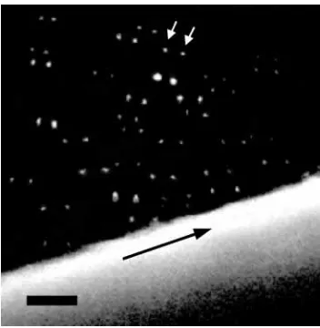
Fluid flow around the fish was illuminated by a horizontal laser sheet, 0.5 mm thick, and imaged from above with a high-resolution digital video camera (Kodak ES 1.0, 1008 pixels×1018 pixels) (Fig. 2). The flow was seeded with neutrally buoyant fluorescent particles, 20–40µm in diameter (Johns Hopkins University). Macro photographic lenses (Nikon, Micro-Nikkor, 60 mm) were used to obtain high-quality, high-magnification images of particles in the flow over the fish surface (Fig. 3). Fields of view used with the particle-imaging camera were 1–2 cm on each side. The resulting images had a scale of 50–100 pixels mm−1. Our fish boundary layers measured 0.5–12 mm in thickness. The laser (New Wave Research, Nd:YAG, dual pulsed) was operated at low power to prevent irritation to the animal and to minimize glare. The time delay, ∆t, between laser pulses, i.e. between exposures of the flow, was set at 2–10 ms depending on swimming speed. The measured displacement of particles between exposures is divided by this time to obtain particle velocities. The laser and the particle-imaging camera were synchronized using a digital delay triggered by every second vertical drive signal of the camera. The vertical drive signal is a TTL pulse that signals the moment between two exposures. When triggered, the digital delay triggered laser 1 of the dual laser to fire ∆t/2 before, and laser 2 to fire ∆t/2 after, the next vertical drive signal of the camera, which was ‘ignored’ by the digital delay. The camera was operated at approximately 30 Hz, and 100 sequential images were acquired per swimming sequence. Therefore, pairs of exposures, or image pairs, were acquired at 15 Hz, and continuous sequences of 50 pairs were acquired. Two standard video cameras were used to obtain simultaneous recordings of whole-body motion in lateral and dorsal views. This allowed fish boundary layer flow to be compared with relevant instantaneous whole-body kinematic variables.
Measurements were confined to positions on the fish where the body surface was essentially perpendicular to the laser
sheet. As the angle between the laser sheet and the fish surface deviates from 90 °, boundary layer velocity profiles are distorted, tending to give an incorrectly low wall shear stress. Images in which the fish surface is perpendicular to the laser sheet are easily distinguished from images in which the surface is at an angle to the sheet. In the former, the fish surface appears as a sharp edge. In the latter, depending on the direction of tilt, either the intersection of the beam and the fish surface is not visible or the features of the fish surface beneath the sheet are visible, dimly illuminated by reflected laser light. Only images of the former type were used in the analysis.
[image:4.612.313.560.71.267.2]In both still-water and flume trials, all three video cameras were fixed with respect to the frame of the test section during image acquisition. In still water, the fish swam through the test section. They therefore swam through each camera’s field of view at their swimming speed, U, and flow velocity outside the fish boundary layer was nearly zero. In the flume, fish held station in the test section without significant streamwise motion with respect to the fields of view. The flow outside the boundary layer of the fish therefore moved through the fields of view at the approximate flume speed, U. Apart from the ambient turbulence of the flume flow, the two situations are equivalent from the standpoint of fluid dynamics. Both techniques proved useful to the analysis of the fish boundary layer. Still-water trials revealed actual boundary layer development over particular fish in undisturbed flow, whereas flume trials revealed the phase-dependent aspects of the boundary layer at selected positions on the fish. The flume was also used to look at boundary layer development by recording several sequences from various streamwise positions.
Fig. 2. Sketch of the experimental arrangement for digital particle imaging velocimetry (DPTV) image pair acquisition. The illustration depicts a still-water trial. U and the arrow represent the velocity of the fish through the test section. In flume experiments, fish were observed to hold station in the flow through the test section. In such cases, U represents the flume speed, and the flume direction would be opposite to the arrow shown.
Dual pulsed laser system High-resolution
digital video camera
Rigid-body drag
In general, the dogfish swam very close to the bottom of the flume, and it was possible to measure the boundary layer of the dogfish at the same streamwise position and flume speed for both swimming and resting. Three image sequences of the dogfish boundary layer were acquired while the dogfish conveniently rested motionless on the bottom of the flume. The flume speed and water temperature were 20 cm s−1and 23 °C. The resting data were used to determine rigid-body friction drag for the dogfish.
It was important to confirm that the bottom boundary layer of the test section did not affect the rigid-body measurements significantly. LDA showed that the boundary layer of the test section bottom was thinner than 1.5 cm. Dogfish boundary layer data were taken between 1.2 and 1.8 cm. Flow visualizations were therefore made outside, or at the outer edge of, the flume bottom boundary layer, where small changes in the height would not be expected to have a significant effect on the flow velocities at the outer edge of the fish boundary
layer, Ue. Velocities measured by particle tracking confirmed this. Uevalues in both the swimming and rigid-body cases were found to be essentially the same at x=0.44L.
Digital particle tracking velocimetry
The acquisition and analysis of image pairs for digital particle image velocimetry (DPIV) and digital particle tracking velocimetry (DPTV) are now common practice among engineers, chemists and a growing number of biologists. For this reason, the details of these techniques will be left to the numerous existing works on the subject; the reader is referred to Adrian (1991), Willert and Gharib (1991) and Stamhuis and Videler (1995). Here, we report the variations on the themes of DPIV and DPTV necessary to capture and resolve the fish boundary layer. Flow velocities around the fish were quantified primarily by semi-automatic DPTV (Stamhuis and Videler, 1995). Particle pairs are located manually with a cursor on the computer screen. The term ‘particle pair’ refers to the two images of the same particle that occur in an image pair. A particular image pair typically has tens to hundreds of particle pairs depending on seeding density. Once the particle pairs have been located, a computer program then determines the centroids of the particles and calculates displacement and velocity. Conventional DPIV and automatic particle-tracking code were sometimes used to resolve the outermost regions of boundary layer flow, but they often failed to resolve the flow very close to the moving surface of the fish.
The fish surface was located using an edge-detection algorithm developed in the study of squid locomotion (Anderson and DeMont, 2000; Anderson et al., 2000). The algorithm was further developed during the course of the present work to match surface features in sequential images and thereby calculate the precise motions of the animal surface. This motion was conveniently described by a tangential and a normal displacement. Deformation and rotation of the fish surface were found to be negligible for any image pair because of the short time separating the images and the small field of view. Trials during which the fish rested motionless on the bottom of the tank revealed the accuracy of this wall-tracking algorithm to be better than 0.5 pixels. At our magnifications, this represents 10–20µm error in displacement and, after smoothing, negligible error in surface slope. For a typical swimming trial, say U=20 cm s−1and ∆t=5 ms, this translates to less than 2 % error in the measurement of tangential flow velocity relative to the fish surface. Average maximum error in normal velocity is 2–10 %, depending on the magnitude of the transverse body velocity. Since wall shear stresses were determined from the slope of the boundary layer profile near the body surface, such errors in velocity relative to the fish surface do not affect our calculated skin friction. Instead, these errors impact less critical measurements, such as outer edge velocity, boundary layer thickness and their fluctuations. In general, these variables were large enough that errors were insignificant to negligible.
Tangential and normal velocity calculations
[image:5.612.86.262.71.251.2]To construct tangential and normal velocity profiles from the Fig. 3. A double exposure showing examples of particle pairs used to
image pairs of flow over the fish surface, the motion of particles in the image pairs must be viewed from the reference frame of the fish. Unless the surface can be described by a straight line, this requires the construction of axes normal and tangential to the fish surface for each particle. Assuming that the velocity profiles do not change significantly over the relatively small field of view, this method results in the desired boundary layer profiles. The separate profiles are built up from the normal and tangential components of velocity determined for each particle, with respect to the fish, plotted against normal distance of the particle from the fish surface.
Normals from particles to the fish surface were determined through a standard minimization of the distances from the particles to the fish surface. The radius of curvature of the fish surface was always larger in scale than the field of view. This ensured convergence of the minimization process. The fish body surface was found to be fitted well by a cubic polynomial. This was used as a means to smooth surface roughness, reducing needless scatter in the minimization process. The normal velocity, v, of a particle with respect to the fish was calculated by:
where ∆t is the time between laser pulses, and y1and y2are the lengths of the normals for the particle in the first and second images respectively. This simple equation can be used because, as mentioned above, the deformation and rotation of the fish surface was negligible over the time between images, ∆t.
The calculation of tangential velocity also began by determining normals to the fish surface from points in the fluid using the same distance minimization. In this case, however, the normals were determined from the midpoint of a particle track to the average position of the fish surface in the two images. The slope of the average fish surface was determined at the intersection of the normal and the average fish surface. The slope was used to construct a unit tangent vector, t, of the average fish surface, in a streamwise sense, with respect to the camera pixel coordinates. That is, the vector lies in the horizontal plane of the laser sheet, is at a tangent to the fish surface and points roughly in the caudal direction. The velocity of the particle, Vp, and the velocity of the fish surface, Vs, were
determined in the same coordinate system. The tangential velocity, u, of the particle with respect to the fish was then determined by the vector operation:
u = (Vp−Vs) · t , (2)
i.e. u is the component of the velocity of the particle, relative to the fish surface, in the direction of the surface unit tangent vector in the plane of the laser sheet. Therefore, u=0 at the fish surface and u=Ueat the edge of the boundary layer. The normal velocity of the particle with respect to the fish can be determined in a similar manner, but normal velocities calculated from equation 1 are more accurate since fish surface averaging is sidestepped. In some instances, conventional DPIV was used to resolve the outer boundary layer and
near-field, reducing the tedium of semi-automatic DPTV processing. The better the seeding, the closer to the fish DPIV could be used with confidence. DPIV nodes were treated as the positions of virtual particles in the first image, and the locations of correlation peaks were treated as virtual particle positions in the second image. This use of DPIV was made only well beyond the linear sublayer of the boundary layer and only when particle densities allowed. The linear sublayer is the region of the boundary layer closest to the body surface in which the tangential velocity profile is linear. It will be shown below that an accurate determination of velocities in the linear sublayer is critical to the analysis of skin friction. As expected in instances of proper seeding, cross checks of such DPIV data by DPTV showed negligible differences in velocities calculated in the outer regions of the boundary layer.
DPTV errors
Absolute errors in DPTV depend on camera pixel resolution, field of view dimensions, particle shape, size, centroid analysis and image quality. Relative errors are magnified by decreased particle displacements, which depend on ∆t and the field of view dimensions. We estimate average maximum DPTV errors of tangential velocities in the linear sublayer of the fish boundary layers to be between 5 and 15 %. This range arises from conservative estimates of sub-pixel accuracy and particle displacements of the order of 10 pixels. These errors tend to be unbiased since they depend on the images of individual particles. Therefore, if enough particle pairs are sampled in a given image pair, the error in wall shear stress determined for that image pair tends to be unbiased. Wall shear stress is determined from a linear fit of the u-profile in the linear sublayer.
Increased scatter was commonly observed in our v-profile data compared with the u-profile data. This is probably due to DPTV errors magnified by generally shorter normal displacements. Turbulence, wall tracking errors, variation in the profile over the streamwise length of the field of view and cross-stream surface curvature may also contribute to scatter in our profiles. In still water, very little scatter was observed in our u-profiles, especially outside the boundary layer, where particles are nearly stationary in the field of view. This is strong support for setting our DPTV error towards the lower end of our estimated 5–15 % mentioned above.
Boundary layer profile analysis
Shapes of actual boundary layer profiles have been determined over the years both theoretically using the Navier–Stokes equations and experimentally using techniques such as hot-wire anemometry. Prandtl’s student Blasius (1908) determined the first boundary layer solution from the Navier–Stokes equations. Blasius (1908) used numerical methods to determine the velocity profiles for the simplest flow geometry – laminar flow over a flat plate with no streamwise pressure gradient. Blasius’ solution shows excellent agreement with experimental data. Since Blasius, several other so-called exact solutions of the Navier–Stokes equations have been determined for laminar boundary layers, including accelerating (1)
and decelerating flows (Falkner and Skan, 1930), and for three-dimensional flows (Sowerby, 1954). It is important to note that these are solutions, not theory, and are, therefore, valid descriptions of boundary layer behavior despite their age.
Knowledge of turbulent boundary layer profiles comes mainly from experimental data. Time-averaged measurements of turbulent flow over flat plates with no pressure gradient have conveniently revealed what is known as the law of the wall (Schlichting, 1979). When appropriately non-dimensionalized, the tangential velocity data follow a universal profile. The effects of streamwise pressure gradients and various geometries on this universal profile are well documented (Schetz, 1993). Tangential velocity, u, and distance from the wall, y, are non-dimensionalized for the law of the wall using the following definitions:
where
ν
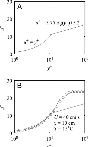
is the kinematic viscosity of the fluid, τois the wall shear stress and ρis the fluid density. The defined intermediate, u*, is known as the friction velocity. Traditionally, the non-dimensionalized tangential velocity, u+, is plotted as a function of log10(y+). Fig. 4A shows the law of the wall plotted in this manner. Two distinct curves are evident. Closest to the wall, which can be thought of as running parallel to the u+axis, the profile is linear, with u+=y+. Note that, on a semi-logarithmic plot, it does not look linear. This curve represents the linear sublayer, which is commonly referred to as the viscous sublayer in the analysis of turbulent boundary layers. Farther from the wall, the profile follows a logarithmic curve. Flow is turbulent in the logarithmic region and laminar in the linear sublayer; a region called the transition zone separates the two. Unlike the linear sublayer, the shape and position of the logarithmic region of the time-averaged profile may very significantly as a result of surface roughness and streamwise pressure gradients (Schetz, 1993). For this reason, data in the logarithmic region cannot be used to determine wall shear stress on an undulating fish. The linear sublayer must be used. Nevertheless, the general shape of the logarithmic region is still useful for distinguishing between turbulent and laminar profiles. Boundary layer profiles were fitted to the law of the wall using the linear sublayer. The profile was then classified as turbulent or laminar on the basis of the profile shape outside the linear sublayer. For example, if the Blasius boundary layer is plotted using the non-dimensionalization of equation 3, the majority of the boundary layer profile follows the linear curve and is poorly fitted by the logarithmic curve (Fig. 4B).It should be noted here that, for turbulent boundary layers, it is the time-averaged profile at a given streamwise position that is described by the law of the wall. This dependence of
the analysis of turbulence on sampling time is due to the fluctuating nature of turbulent flow. If the sampling time is too short, the instantaneous boundary layer profile could appear to be laminar – and not necessarily Blasius-like – even if the flow were turbulent. It is only when several instantaneous boundary layer profiles over a particular point in a turbulent boundary layer are drawn overlapped that the average curve drawn through the combined profiles follows the law of the wall. Our profiles, at most, can be considered time averages over an effective sampling period of Ts=l/U, where l is the streamwise dimension of the field of view and U is the swimming speed. Tsin our experiments ranged from 0.02 to 1.0 s, much shorter than traditional sampling periods, and led to uncertainty in the designation of certain profiles as turbulent. Nevertheless, several of our fish boundary layer profiles at high Reynolds (3)
u u* u+≡
u*≡
,
冪
τo ρyu *
ν
y+≡100 101 102
0 10 20 30
u
+
y+
u+ = 5.75log(y+)+5.2
u+ = y+
A
100 101 102
0 10 20 30
y+
u
+
U = 40 cm s-1 x = 10 cm T = 15°C
[image:7.612.369.520.75.328.2]B
numbers showed excellent agreement with the law of the wall. More importantly, in the neighborhood of a particular surface position, the shapes of u-profiles in the linear sublayer of a turbulent boundary layer are less variable than those in the logarithmic region. Therefore, it is safe to assume that our measurements of wall shear stress, which are based on the linear sublayer, are accurate.
Throughout the discussion of the measured boundary layers, the quantity, Rex, or the ‘length Reynolds number,’ is used. Rex is the Reynolds number based on position, x, i.e. Rex≡Ux/
ν
. Rexis commonly used (Fox and McDonald, 1992) in detailed analyses of fluid phenomena that depend on streamwise position, such as boundary layer thickness, wall shear stress and the transition of boundary layer flow from laminar to turbulent. For example, the position at which laminar flow makes the transition to turbulent flow over a flat plate does not depend on the total length, L, of the plate. Instead, transition tends to occur at Rex=3.5×10⁵to 5×10⁵, for any flat plate or relatively similar surface (Schlichting, 1979), regardless of L and, subsequently, the standard Reynolds number based on length, Re. Note that Rexat x=L is the same as Re.Wall shear stress and friction drag
The tangential component of wall shear stress, τo, in the plane of the laser sheet was determined using:
where µ is the dynamic viscosity of the fluid, u=u(y) is the tangential component of fluid velocity over the object in the plane of the laser sheet and y is in the direction of the local outward normal of the surface. In the linear sublayer of both laminar and turbulent boundary layers, the value of the partial derivative – the normal gradient of u – is constant and can be determined by a simple linear fit. This use of experimental data to determine wall shear stress has been termed the ‘near-wall method’ by Österlund and Johansson (1999). Their wall shear stresses calculated from equation 4 using hot-wire velocity measurements show excellent agreement with theory and concurrent measurements of shear stress by the oil-film technique. They also determined and verified fluctuating shear stress measurements, due to the unsteadiness of turbulent flow, with Micro Electro Mechanical Systems (MEMS) hot films.
The wall shear stress distribution, τo, over an object can be used to calculate the total friction drag, Df, using:
where S is the three-dimensional function defining the body surface of the fish, dA is the incremental area over which a particular shear stress applies, and θis the angle between the body surface tangent in the laser plane and the streamwise direction. The coefficient of friction for any object is defined as:
where ρis the fluid density, A is the total wetted surface area of the body and U is the relative velocity of the object through the fluid. To obtain accurate values of friction drag and the coefficient of friction for a swimming fish, a large number of measurements of wall shear stress at different positions and at different phases of the undulatory motion must be taken.
For comparative purposes, a local coefficient of friction, Cfx, was defined as:
By this definition, Cfis the area average of Cfxover the fish surface. Therefore, Cf for a given fish falls between the maximum and minimum values of Cfxdetermined over the fish body. Rough time averages of Cfx and other boundary layer variables were determined by simply averaging these quantities over sufficient boundary layer realizations to cover the entire locomotory cycle.
Undulatory phase
Boundary layer data were taken on one side of the fish for any given trial. The fish surface oscillated in the field of view of the particle-imaging camera because of the transverse motion of the body. We will use the term ‘crest’ to describe the instance when the section of the fish surface in view has moved to its full amplitude in the direction of the outward-pointing surface normal, i.e. the positive y-direction. We use ‘trough’ for the instance of full amplitude in the negative y-direction. Phase is set to 90 ° at the crest and 270 ° at the trough. Transverse wall velocity as a function of time determined from wall tracking was fitted with a sine function. The phase of the body surface transverse position was determined by integrating wall velocity or simply by subtracting 90 ° from the phase of transverse wall velocity.
Detailed phase analysis was only applied to flume data. Still-water trials result in a more complicated mix of phase and position. The propulsive wave of the fish travels streamwise at a speed slightly greater than the swimming speed, U (Gray, 1968). Since, for still water, the field of view is fixed with respect to the bulk fluid in the tank, phase appears to change more slowly than if observed in a flume. If the wave speed were nearly equal to the swimming speed, almost no change in phase would be observed. Therefore, still-water trials give information at various phases at various positions. In contrast, flume trials give information at one position as a function of phase.
Results
Fish boundary layer profiles
More than 70 swimming sequences of scup and 30 sequences of dogfish were acquired, yielding hundreds of usable image pairs for boundary layer realization. Tangential (7)
τo GρU2,
Cfx≡
(6) Df
GρAU2,
Cf=
⌠
⌡τodAcosθ, (5)
Df= ⌠ ⌡
S
(4)
τo=µ ,
y=0
∂u
and normal velocity profiles were determined for more than 270 image pairs from 36 swimming sequences with high image quality over the full range of experimental speeds. Only one dogfish has so far been examined, so generalizations concerning anguilliform swimmers must be considered tentative. Nevertheless, the quantity and consistency of the dogfish data suggest that the conclusions regarding the specimen observed are well founded.
Fish boundary layer profiles tended to resemble the solutions of either Blasius or the law of the wall (Fig. 5). Profiles that deviated from these two types often exhibited good agreement with the Falkner–Skan solution (Fig. 6). The Falkner–Skan solution can describe either an accelerating (Fig. 6A,B) or a decelerating (Fig. 6C,D) boundary layer depending on the choice of a coefficient in the Falkner–Skan differential equations. Boundary layers are classified as accelerating or decelerating on the basis of their u-profiles. However, in the instantaneous profiles of a boundary layer, the evidence of acceleration or deceleration is found in the v-profile. Negative normal velocity at the outer edge of the boundary layer (Fig. 6B) reveals that there is a net normal flow of fluid, or normal flux, into the boundary layer characteristic of an accelerating boundary layer. In contrast, the Blasius solution always shows positive normal velocity at the edge of the boundary layer (Figs 5B, 6B) and is, therefore, a decelerating boundary layer.
The connection between normal flux and acceleration involves the incompressibility and continuity of water. Imagine a constant-diameter pipe carrying water with a prescribed
upstream volume input. If the pipe is tapped, so that water can be pumped in or out, the downstream volume flow of the pipe can be changed. Incompressibility and continuity require that the flow speed must also change. If water is pumped in, flow must accelerate in the pipe in the vicinity of the tap. If we pump water out, the pipe flow decelerates.
Fish boundary layer profiles occasionally resembled strongly decelerating Falkner–Skan profiles characterized by highly inflected u-profiles with low wall shear stress (Fig. 6C). The v-profiles of these realizations revealed flow out of the boundary layer characteristic of boundary layer deceleration (Fig. 6D). Inflected boundary layers of this type are often a sign of incipient separation (Batchelor, 1967). No profiles indicative of separation were observed.
Flow condition in the boundary layer
In still-water trials, boundary layer profile shapes always suggested laminar flow. This is not entirely surprising since Reynolds numbers, Re, were 3×10³ to 6×10⁴ lower than the standard critical range for boundary layer transition, Rex=3.5×10⁵to 5×10⁵. Recall that, at x=L, Re
xis at a maximum and equal to Re. In flume trials, however, both laminar and turbulent profile shapes were observed even though Reynolds numbers did not quite reach the critical value. The critical values for boundary layer transition assume quiet incoming flow over smooth rigid surfaces. The ambient turbulence of the flume, the roughness of the fish surface and the unsteadiness of the flow over the fish might be expected to trip turbulence at lower than critical Reynolds numbers. The boundary layer Fig. 5. Two representative boundary layer
realizations illustrating the distinction between laminar-like and turbulent-like boundary layers. Each data point represents information calculated from one particle pair of the image pairs used for the given realizations. The first realization shown (A–C) is from x=0.50L, where L is body length, on a scup swimming in the flume at 42 cm s−1, Rex≈4×10⁴. The second (D) is from x=0.53L on the dogfish swimming in the flume at 20 cm s−1, Rex≈4×10⁴. (A) The u-profile of the first realization showing agreement with a Blasius fit drawn as a solid curve. (B) The v-profiles of the first realization and the Blasius fit of A. (C) The u-profile of the first realization compared with the law of the wall by fitting the linear sublayer. The boundary layer distinguishes itself as laminar-like, as outlined in Fig. 4. (D) The dogfish boundary layer realization showing good agreement with the law of the wall, distinguishing the profile as turbulent-like. Note the slight shift in the logarithmic region. The fit exhibits sharp contrast to the fit of the profile shown in C. Rex, the length Reynolds number based on x, the
streamwise position on the body measured from the leading edge; u, tangential velocity; y, normal distance from the body surface; v, normal velocity; u+, y+, non-dimensionalized tangential velocity and normal distance, respectively.
0 10 20 30 40 50
0 1 2 3
u (cm s-1)
y (mm)
A
-20 -10 0 10 20
0 1 2 3
v (cm s-1)
y (mm)
B
100 101 102
0 10 20 30
y+
u
+
C
100 101 102
0 10 20 30
y+
u
+
[image:9.612.251.565.75.341.2]over scup swimming in the flume at 30 cm s−1, Re=6×10⁴, was apparently always laminar over the entire body. The boundary layer over a dogfish swimming at 63 cm s−1, Re=3×10⁵, measured at x=0.63L, Rex=1.9×10⁵, appeared to be primarily turbulent. In some cases, at Reynolds numbers between these two values, the boundary layer apparently oscillated between laminar and turbulent. When this was observed, turbulent profile shapes tended to appear at the crest phase of the body wave. The boundary layer generally returned to a laminar shape during the crest-to-trough motion.
The rigid-body case of the dogfish revealed an interesting effect. Flow appeared laminar at x=0.44L and turbulent at x=0.69L. For the swimming dogfish, boundary layer flow appeared to be laminar at x=0.44L and x=0.69L for most of the time, with some evidence of oscillation between laminar and turbulent flow at x=0.69L. The observation of laminar boundary layer flow at x=0.69L during swimming suggests a stabilization process. The same phenomenon was observed by Taneda and Tomonari (1974) comparing the boundary layer flow for the rigid body and various swimming cases of a waving plate.
Local friction coefficients
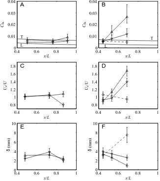
Posterior to x=0.8L in scup and x=0.5L in dogfish, the time-averaged local friction coefficients, Cfx, of both species increase above the flat-plate laminar and turbulent values (Figs 7, 8). This increase in friction is much more dramatic in the anguilliform swimmer. Local friction coefficients in the rigid-body case of the dogfish do not show this increase and remain between the laminar and turbulent flat-plate values, i.e. the friction drag on the swimming dogfish is higher than that on the dogfish stretched straight in the flow.
In many cases, the values of Cfx, Ueand δ versus relative
u (cm s-1)
y (mm)
v (cm s-1)
y (mm)
u (cm s-1)
y (mm)
v (cm s-1)
y (mm)
0 10 20 30
0 1 2 3
A
-5 0 5
0 1 2 3
B
0 5 10 15
0 2 4 6 8
C
-2 -1 0 1 2
0 2 4 6 8
[image:10.612.263.563.73.326.2]D
Fig. 6. Two representative boundary layer realizations that are fitted well by the Falkner–Skan solution. The first realization (A,B) is from x=0.50L, where L is body length, on a scup swimming in the flume at 30 cm s−1, Rex≈3×10⁴. The second (C,D) comes from very close to the body trailing edge of a scup swimming in still water at 14 cm s−1 and decelerating at 10 cm s−2, Rex≈2×10⁴. (A) The u-profile of the first realization with a Falkner–Skan fit drawn as a solid curve. The dashed curve is the Blasius solution with the same wall shear stress. (B) The v-profiles of the first realization, the Falkner–Skan solution and the Blasius solution. (C) The u-profile of the second realization. (D) The v-profile of the second realization. The solid curve is the Falkner–Skan fit. Rex, the length Reynolds number based on x, the streamwise position on the body measured from the leading edge; u, tangential velocity; y, distance from the body surface; v, normal velocity.
2×10⁴ 4×10⁴ 6×10⁴ 8×10⁴
10-3 10-2 10-1
L T
Rex Cfx
[image:10.612.54.283.345.515.2]position, x/L, were observed to depend both on species and on the sign of the transverse velocity of the fish surface (Fig. 8). Cfx increases out of the range of flat-plate friction more forward on the body of the dogfish than on the scup (Fig. 8A,B). In both species, local friction oscillates in phase with transverse body velocity (Fig. 8A,B). In the dogfish, the time average of Ueincreases with streamwise position on the body (Fig. 8D), suggesting a mean acceleration of both the boundary layer and the near-field flow over the fish. In the scup, the time average of Ueis close to U for the entire region that was measured (Fig. 8C). In both species, Ueoscillates in phase with transverse body velocity (Fig. 8C,D) and local friction (Fig. 8A,B), suggesting local oscillatory acceleration and deceleration in the near-field and boundary layer. The boundary layer thickness over the posterior region of the dogfish, where local friction increases above flat-plate friction, oscillates 180 ° out of phase with transverse body velocity (Fig. 8F). Oscillatory effects in Cfx, Ueand δare more pronounced in the anguilliform swimmer than in the carangiform swimmer. Finally, the behavior of Cfx, Ueand δin the rigid-body case is opposite to that in the swimming dogfish (Fig. 8B,D,F), while scup data show some similarity to the rigid dogfish case.
Uncertainties in Cfx, Ue and δ were determined to be
approximately ±31 %, ±6 % and ±21 %, respectively, with some variation among trials depending on the quality of the flow realizations. For example, the rigid-body case of the dogfish has lower than average uncertainty in Cfx(±19 %) as a result of the large number of images of the same event acquired; i.e. many particle pairs were sampled. Uncertainties were often greater in one direction than another. For instance, the uncertainties in Cfxfor the swimming dogfish were +42 % and −21 %. Where appropriate, error bars are used to display the unique uncertainties of data points.
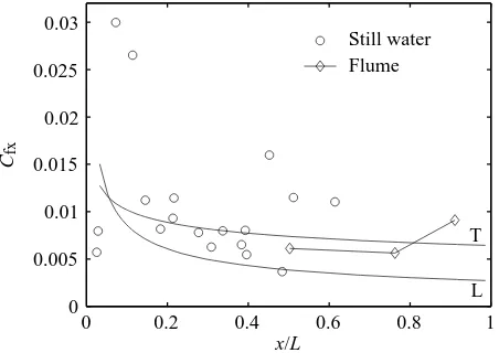
Data from scup swimming in the flume at swimming speeds ranging from 30 to 60 cm s−1at a water temperature of 23.3 °C show that, in the neighborhood of x=0.5L, Cfxfalls within the range of values expected for flat plates (Fig. 9). The effects of transverse body surface velocity at this position are consistently small compared with more caudal positions (Fig. 8A). Therefore, at some positions on the fish, Rexappears to be sufficient to predict local friction, whereas at other positions local friction deviates from flat plate friction and oscillates significantly. Boundary layer data from still-water trials in scup suggest that the similarity to a flat plate may extend over the majority of the anterior half of the fish (Fig. 10). Boundary layer acceleration due to the finite
0.4 0.6 0.8 1
0 0.01 0.02 0.03 0.04
x/L
Cfx
A
L T
0.4 0.6 0.8 1
0 0.01 0.02 0.03 0.04
x/L
Cfx
B
L
T
0.4 0.6 0.8 1
0.8 1 1.2 1.4 1.6 1.8
x/L
Ue
/U
C
0.4 0.6 0.8 1
0.8 1 1.2 1.4 1.6 1.8
x/L
Ue
/U
D
0.4 0.6 0.8 1
0 2 4 6 8 10
x/L
δ
(mm)
E
0.4 0.6 0.8 1
0 2 4 6 8 10
x/L
δ
(mm)
[image:11.612.243.569.74.443.2]F
thickness of the scup leading edge, in contrast to a flat plate, is the likely explanation of a spike in local friction observed near the anterior end (Fig. 10).
Oscillatory behavior of the boundary layer
Oscillations in Cfx, Ueand δ were highly correlated to the transverse velocity of the body surface (Fig. 8). Local friction and Uetend to be highest when the fish surface is moving into the fluid and lowest when the surface is retreating from the fluid; δbehaves in the opposite manner. A more highly resolved picture of the relationships between Cfx, Ue, δ and Ve versus body phase was obtained using polar phase plots for the dogfish swimming at 20 cm s−1(Figs 11, 12). C
fxand Ueare roughly in phase. Boundary layer thickness is roughly 180 ° out of phase with Cfx. Normal flux oscillates roughly 180 ° out of phase with transverse body velocity. In addition to these previously described trends, the phase plots reveal a clockwise procession of maximum Cfx, Ue, δand possibly Vewith increasing relative position, x/L. This procession suggests that the distributions of these variables can be characterized as waves travelling along the body of the fish with wavelengths and speeds different from those of the body wave. The details of these ‘distribution waves’ will be discussed below.
Oscillation of normal velocity
Not only was Veobserved to oscillate with body motion, but sequences of normal velocity profiles in both scup and dogfish swimming in the flume also revealed oscillation throughout the entire profile (Fig. 13). In both species, the sign of the normal
velocity throughout the boundary layer is 180 ° out of phase with transverse body surface velocity, vw. As the body surface moves into the fluid, normal velocity is negative. During retreat, it is positive. At this short distance from the surface of the fish, incompressibility and continuity predict that this behavior is not simply a relative velocity effect. Furthermore, if the effect were due strictly to relative motion, the v-profiles would be expected to exhibit velocities equal to the transverse wall velocity throughout the boundary layer.
Incipient separation
While no boundary layer separation was observed in the fish studied, incipient separation was seen in six swimming sequences. Figs 14 and 15 show examples of incipient separation in scup in both still and flowing water. The example from still water (Fig. 14) dramatically demonstrates the highly inflected, low shear boundary layer profile shape of incipient separation. Our data show that incipient separation occurs after wall velocity, vw, becomes negative, and that friction essentially drops to zero where the inflected profiles occur.
[image:12.612.52.286.53.242.2]In the flume, a time sequence of the boundary layer behavior was obtained that included incipient separation (Fig. 15). As in the still-water example (Fig. 14), incipient separation occurs close to where wall velocity, vw, becomes negative. Local friction decreases noticeably. The time sequence suggests that the inflected boundary layers, which occur at troughs, are stabilized as the body phase cycles towards the subsequent crests. In the flume, instances of inflected boundary layers were observed twice in separate sequences of scup swimming at 30 cm s−1and once in the dogfish swimming at 20 cm s−1. Fig. 9. Time-averaged local friction coefficients, Cfx, versus length
Reynolds number, Rex, at x=0.50L, where L is body length, from several scup swimming sequences ranging in swimming speed from 30 to 60 cm s−1. No lines are drawn connecting these data points (diamonds) since they do not represent the distribution of coefficients of friction along the body of a scup. The data at each Rex represent 9–10 boundary layer realizations. Error bars are based on the maximum percentage errors in the determination of the slope of the linear sublayer, i.e. the wall shear stress, for the boundary layer profiles contributing to each data point. Rex, the length Reynolds number based on x; x, position along the body.
L T
2×10⁴ 4×10⁴ 6×10⁴ 8×10⁴
10-3 10-2 10-1
Rex Cfx
0 0.2 0.4 0.6 0.8 1
0 0.005 0.01 0.015 0.02 0.025 0.03
Cfx
x/L
T
L Still water Flume
[image:12.612.325.551.73.233.2]Total skin friction and friction coefficients
Table 1 presents calculations of total body friction drag and corresponding friction coefficients for scup (swimming) and dogfish (swimming and rigid). The power required to overcome friction drag is also presented. In Fig. 16, the coefficients of friction are plotted versus Re together with flat-plate friction for comparison. The coefficients of friction for swimming scup and the rigid dogfish fall within the range of flat-plate friction for laminar and turbulent flow. The coefficient of friction for the swimming dogfish lands above this range.
Discussion
The nature of the fish boundary layer
In the most general sense, the boundary layer of swimming fish can be characterized by streamwise trends and local
oscillations in Cfx, Ue, δ, Ve and overall profile shape. Streamwise trends proved to be highly dependent on swimming mode (Fig. 8). Local oscillations of boundary-layer-related variables occurred similarly in both the dogfish and scup, although the amplitudes of oscillation were greater in the dogfish. The data reveal that all these behaviors can be understood from the perspective of two superimposed fluid accelerations: mean streamwise acceleration and local oscillatory acceleration that is correlated to the transverse motion.
[image:13.612.88.535.73.370.2]The streamwise increase of Uein the dogfish is evidence of mean streamwise acceleration of the near-field and boundary layer flow. The time-averaged values of Cfx increase and of δ decrease, as would be expected in a boundary layer under an accelerating exterior flow. No significant mean streamwise acceleration was observed in scup; however, the near-field flow Fig. 11. Phase plots of local friction coefficients, Cfx, and boundary layer thickness, δ, from 10 swimming sequences of the dogfish at the same swimming speed, U=20 cm s−1, at three streamwise positions, representing 100 boundary layer realizations. The three positions along the body examined were, x=0.44L, 0.53L and 0.69L, where L is body length. Each phase plot presents the behavior of a particular boundary layer variable versus body phase,φ, measured at a particular position along the fish. The crest of the body surface corresponds to φ=90 °; the trough corresponds to φ=270 °. Time and phase increase in the counterclockwise direction, and radial distance expresses the magnitude of the boundary layer variable plotted. The radial scaling is printed between the angular positions 60 and 90 °. A solid radius is drawn on each phase plot to mark the phase of the maximum value of the variable displayed. Consider the plot of Cfxat x=0.69L. At φ=0 °, the body is cycling from trough to crest, and Cfxis equal to 0.033. The highest positive transverse body velocities occur near this phase. As the phase reaches 90 °, the body reverses direction. Cfxdecreases, reaching a minimum of 0.005 near φ=150 °. At the trough, φ=270 °, friction is increasing and reaches a maximum near φ=330 ° as the body is thrust towards the fluid. The cycle then repeats itself. The set of three plots for each variable are drawn to the same scale so that magnitudes as well as phase relationships can be compared. For example, one can observe the mean streamwise increase in Cfx, noting the progressive increase in area enclosed by the plotted curves. These curves are fourth-degree polynomial fits of the boundary layer data. They are constrained to be periodic, but not sinusoidal, by equalizing function values and slopes at the beginning and end of the cycle. This method of fitting the data allows for asymmetric phase plots.
Cfx
0.02 0.04
30°
210°
60°
240° 90°
270° 120°
300° 150°
330°
180° 0°
0.02 0.04
0.02 0.04
x = 0.44L
δ
(mm)
2.5 5
x = 0.53L
2.5 5
x = 0.69L
2.5 5
30°
210°
60°
240° 90°
270° 120°
300° 150°
330°
180° 0°
30°
210°
60°
240° 90°
270° 120°
300° 150°
330°
180° 0°
30°
210°
60°
240° 90°
270° 120°
300° 150°
330°
180° 0°
30°
210°
60°
240° 90°
270° 120°
300° 150°
330°
180° 0°
30°
210°
60°
240° 90°
270° 120°
300° 150°
330°
was not observed to decelerate either. The absence of mean acceleration over the scup follows from the tendency of carangiform swimmers to produce the majority of their thrust at the caudal fin. Mean streamwise acceleration is a sign of thrust production anterior to the caudal fin. The difference between scup and dogfish in this regard can be understood by considering the relatively small wave amplitudes present in carangiform swimmers. Studies of swimming performance after complete caudal fin amputation (Breder, 1926; Gray, 1968; Webb, 1973) show that carangiform swimmers are able to compensate surprisingly well for the loss of fin thrust by increasing body wave amplitude and frequency. The observed differences in amplitude and frequency after complete amputation suggest a change in swimming mode on the part of the fish. Mean streamwise acceleration of the near-field might be expected to occur over a larger portion of the body in these fish since they have only their bodies to produce thrust in the amputated state. However, it does not follow that carangiform swimmers actually do use their body wave to produce a significant amount of thrust forward of the caudal fin. When the caudal fin is amputated, one would not expect the fish to use the same body motion to swim as it did with the caudal fin intact. Therefore, it would be tenuous to conclude that, since a carangiform swimmer with its caudal fin amputated uses body-based thrust to swim, the same is true when the tail has not been removed. Our data suggest low body-based thrust in scup compared with caudal-fin-body-based thrust since mean streamwise acceleration of the near-field fluid forward of the peduncle, which would be the evidence of the body producing thrust forward of the peduncle, was not observed.
In both scup and dogfish, Ueand δwere observed to oscillate 180 ° out of phase with each other. Cfxbehaves as would be expected according to the first-order approximation τo≈µUe/δ (equation 4). This and the concurrent oscillation of the v-profile
(Fig. 13) reveal a cycle of local tangential acceleration and deceleration of the boundary layer at any given position along the fish. As explained above, positive and negative normal velocity relative to the body at the edge of the boundary layer are evidence of normal flux out of and into the boundary layer, respectively. In general, tangential flow accelerates as the body cycles from trough to crest, and decelerates as the body cycles from crest to trough.
One might argue that normal flux exhibited by the v-profile is simply the observation of relative motion due to the surface-fixed coordinate system, but that would be true only if one were focusing on the far-field, where there is negligible impact on the flow due to the fish. Allen (1961) apparently uses this far-field concept to explain his supposed observation of boundary layer thickness oscillation. In contrast, the normal flux revealed in Fig. 13 occurs at the level of the near-field and boundary layer. Therefore, it is not merely relative fluid motion. This is indicated by the fact that across the boundary layer, normal velocity, v, remains well below vw in magnitude. Near the surface of the fish this is the necessary result of the continuity and incompressibility of water and the no-flux boundary condition at the surface. The fact that the same is observed at the edge of the boundary layer indicates tangential and/or cross-stream boundary layer acceleration.
Wave-like distributions of boundary layer variables and pressure
[image:14.612.45.561.95.317.2]As mentioned above, the oscillatory behavior of Cfx, Ue, δ and Ve with relative position along the fish suggests that the streamwise distributions of these variables can be represented as travelling waves moving in the same direction as the fish body wave. The clockwise procession of maximum values in the phase plots reveals an ever-increasing downstream shift in Table 1. Total drag calculations based on measured wall shear stress distributions over scup Stenotomus chrysops and dogfish
Mustelus canis
M. canis S. chrysops
Flume, rigid body Flume Still water Flume
Swimming speed, U (cm s−1) 20 20 10 30
Temperature, T (°C) 22.8 22.8 23.3 23.3
Lateral body area, A (m2) 0.0213 0.0213 0.0206 0.0206
Body length, L (cm) 44.4 44.4 19.5 19.5
Mass, M (kg) 0.218 0.218 0.166 0.166
Measured friction drag, Df(N) 0.0033 0.0064 0.0013 0.0067
Theoretical rigid-body friction drag, Dft(N) 0.0018 0.0018 0.0007 0.0044
Measured friction drag coefficient, Cf 0.0076 0.0146 0.0127 0.0071
Theoretical friction drag coefficient, Cft 0.0041 0.0041 0.0068 0.0047
Df/Dft 1.8 3.6 1.9 1.5
Df/measured rigid-body friction drag 1.0 1.9
Power required to overcome Df(mW) NA 1.3 0.13 2.0
Mass of red muscle per mass of fish 0.0209*
Mass of red muscle (kg) 0.0035
Power required per mass red muscle (W kg-1) 0.6
the streamwise distributions of these variables with respect to the phase of the body travelling wave (Figs 11, 12). The regular periodic behavior of these variables at fixed positions on the fish reveals that these ‘distribution waves’ and the body travelling wave have the same frequency, f. Since c=λf, the increasing streamwise phase shift of the variable distributions with respect to the body wave is therefore due to the distribution waves having a longer wavelength, λ, and higher wave speed, c, than the body travelling wave.
Wave speeds and wavelengths of the distribution waves can be determined from the streamwise rate of procession. The procession of local friction is approximately 30 ° as x changes from 0.44L to 0.53L. Between x=0.53L and 0.69L, procession is approximately 60 °. Therefore, the ratio of procession to change in body position, i.e. the rate of procession, is roughly constant (approximately 354 ° per body length). Thus, the wavelength and wave speed of the streamwise distribution of local friction are roughly constant. If the rate of procession with streamwise position were variable, the wavelength and wave speed would be variable. In the dogfish swimming at 20 cm s−1, the measured body wavelength, λ, was 27 cm and body length, L, was 44.4 cm. Therefore, the rate of procession given above translates to approximately 215 ° per body wavelength, i.e. when the body wave travels one body wavelength, the friction distribution travels 1.6 body
wavelengths. In other words, the friction distribution travels 1.6 times faster along the body than the body wave. Boundary layer thickness exhibits the same rate of procession. Ueappears to have the same rate of procession despite the larger phase shift between x=0.44L and 0.53L. There is so little variation in Ueat x=0.44L that it is possible that there is significant error in the determined phase of the maximum. Finally, normal flux, Ve, exhibits the same rate of procession between x=0.44L and 0.53L, but very little procession occurs between x=0.53L and 0.69L.
[image:15.612.90.534.73.369.2]Taken together, the general procession of all four variables (Figs 11, 12) is evidence of a travelling pressure distribution over the fish. Boundary layer thinning, negative normal flux and the increase in Uecan be understood as being linked to accelerations of the boundary layer and near-field flow. These accelerations, in turn, can be thought of as being driven, at least in part, by pressure gradients. We assume here that maxima in boundary layer acceleration, as shown by Cfx, Ue, δand Ve, are indicative of maxima in pressure gradient. Therefore, the pressure distribution around the fish behaves like the distributions of these variables in wavelength and wave speed. From this assumption, the data in Figs 11 and 12 suggest that the travelling wave of the pressure distribution and the body wave are approximately 60 ° out of phase at x=0.44L, with pressure lagging behind the body wave. This means that, when Fig. 12. Phase plots of tangential and normal velocity at the edge of the boundary layer, Ueand Ve, respectively, for the same 10 swimming sequences of dogfish swimming (20 cm s−1) as in Fig. 11. The details of the construction of the phase plots are described in the legend of Fig. 11. For Ve, the solid lines represent positive values, or outflow, and the dashed lines, negative values, or inflow. The increasing area enclosed by the plots of Ueshow mean streamwise acceleration as shown in Fig. 8D.
17.5 35
17.5 35
17.5 35
Ve
(cm s
-1) Ue
(cm s
-1)
1.3 1.3
2.6
1.3 2.6 30°
210°
60°
240° 90°
270° 120°
300° 150°
330°
180° 0°
x = 0.44L x = 0.53L x = 0.69L
30°
210°
60°
240° 90°
270° 120°
300° 150°
330°
180° 0°
30°
210°
60°
240° 90°
270° 120°
300° 150°
330°
180° 0°
30°
210°
60°
240° 90°
270° 120°
300° 150°
330°
180° 0°
30°
210°
60°
240° 90°
270° 120°
300° 150°
330°
180° 0°
30°
210°
60°
240° 90°
270° 120°
300° 150°
330°
180° 0°