Realistic route choice modeling

(1)

MASTER THESIS REPORT

Author:

M.G. T

ELGEN

BS

C

Date:

June 17, 2010

Supervisors:

DHV:

Ir. M.C.VERKAIK-POELMAN

Civil Engineering and Management:

Prof. Dr. E.C.

VAN

BERKUM

Dr. R.PUEBOOBPAPHAN

(2)

(3)

Acknowledgements

A human life is a chain of decisions, important decision, but also day-to-day decision like what to wear. This year, I made a lot important decisions. I decided to move to Utrecht and moved in with my boyfriend Niels. I decided to do my confession of faith, and this year I decide to which jobs I want to apply. All important decisions, which I could not make if I did not get the opportunities for them. I am grateful for all the oppor-tunities I received. I would like to thank the people responsible for the opporoppor-tunities I received in regarded to performing this master thesis project.

First of all I thank my parents for supporting me. Thank you for supporting me in my decisions, and for giving me all the opportunities to follow two study programs.

I would like to thank Muriel Verkaik-Poelman for supporting me during the master thesis project. You did not only represent the DHV vision on my research project, but you also kept in mind what is reasonable to expect from me, and helped me with the problems I encountered.

I would also like to thank my supervisors of the University of Twente. Eric van Berkum thank you for helping me finding a master thesis project, and advising during the research project. Rattaphol Pueboobpaphan thank you for supporting me during the project, and helping me focus the research goal in a more realistic research goal. Judith Vink-Timmer thank you for supporting me in my master thesis project, and helping me with the proofs. Werner Scheinhardt thank you for reading my master thesis project, and your comments.

Finally I would like to thank Niels for supporting and advising me in my decisions. Niels I want to thank you for helping me with the English language and listen to my stories, but more importantly I want to thank you for being there for me.

In the remaining of this report I will focus on the choices rather than on the opportunities.

(4)

(5)

Summary

Traffic engineers use transport models to predict future traffic streams. The route choice model is an impor-tant step of the transport model. We observe unrealistic routes in the results of the transport models used at DHV. But DHV has never calibrated or validated their transport model with regard to the route choices. From all the steps of the transport model we expect the biggest improvement of the transport model by improving the route choice model. DHV often uses the shortest route principle. We investigate literature for other route choice models.

We found several promising route choice models besides the shortest route principle. We select the most promising route choice models on the basis of: reality, computational time, and ease of use. The C-logit and the game theory based route choice models are realistic route choice models with reasonable computational time, and are easy to use due to earlier experience with these approaches. We select both approaches for fur-ther investigation. Within the C-logit we vary different parameter values, including the scale parameter. We vary the scale parameter, because we proved that the C-logit results depend on the utility scale. The games of game theory we use are the congestion game, the demon player game, the smooth fictitious play under the Multinomial logit rule, and the smooth fictitious play under the C-logit rule. In literature, the smooth fictitious play is only described under the Multinomial logit rule. We verify the use of the C-logit by a proof of conver-gence of the smooth fictitious play under the C-logit rule.

We formulate our research goal to investigate these two route choice model approaches:

Investigate whether route choice models based on C-logit and game theory are able to produce more realistic route choices than the shortest route principle, and investigate the behavior of the C-logit and game theory models.

We define the measure reality to express the extent in which a variant produces realistic route choices. The reality of a route choice model is the percentage of vehicles that chooses the same route according to the route choice model and loading method as registered by data, where we assume that the transport model generates the same amount of vehicles in the network as registered. We calculate in four different tests the reality scores of the C-logit and game theory variants with different parameter settings, and the reality score of the shortest route principle. We compare the reality scores with each other to determine the influence of the parameters on the C-logit and game theory, and whether the C-logit and game theory based route choice models are able to produce more realistic route choices. We only test on short trips (less than 11 km), therefore we cannot draw conclusions about our route choice models with long trips.

The tests results make clear that C-logit and game theory based route choice models can produce more re-alistic route choices than the shortest route principle. We expect that the C-logit and game theory based route choice models also result in more realistic route choices than the shortest route principle for other than our tested network, because the reality scores of the most C-logit and game theory variants where much larger than the reality scores of the shortest route principle on all the tested origin destination pairs.

The parametersβ,θ, and the penalty function seem not to have much influence on the C-logit results when multiple origin destination pairs are used. We expect that this result also holds for other networks when using multiple origin destination pairs, because the tests show that other parameter settings are optimal for different origin destination pairs. These differences can level each other out if the C-logit is used on multiple origin des-tination pairs. The power of the travel time has very small influence on the C-logit results. The commonality factor has more influence, and the results indicate that commonality factor 4 is the most realistic commonality factor. We believe that commonality factor 4 is in general the most realistic commonality factor, because com-monality factor 4 scores the highest reality score on all our tests with all parameter settings.

The distance fraction has not much influence on the route choices of the congestion game, unless we use un-reasonably large distance fractions. Theβ,θ, commonality factor, and penalty function show similar behavior with the C-logit as with the smooth fictitious play. We are not able to model the demon player game in a dynamic assignment with reasonable computational time, therefore we did not test the demon player game in a dynamic assignment.

(6)

6

(7)

Chapter 1

Introduction

This report describes the master thesis project of Marthe Telgen. Marthe Telgen performed her master thesis project at DHV. DHV is active in consultancy and engineering in Europe, Asia, Africa, and North America. DHV services on the markets transportation, water, building & industry, and spatial planning & environment. Marthe Telgen performed her project at the unit environment and transportation in Amersfoort. About 120 people work in this unit. The unit is divided into four different departments: transport models, urban & regional mobility, dynamic traffic management, and mobility consultancy. Marthe Telgen performed her thesis project at the department traffic models.

1.1

Research subject

The department transport models works with various kinds of transport models. A transport model is used to predict the influences of traffic measures, construction plans, or demographical changes on traffic streams. The transport models consist of several sequential steps. The route choice is one of the steps in a transport model. Errors in the route choice step will cause errors in the prediction of the total model. DHV recognizes that the transport models currently used at DHV do not always result in realistic routes. We believe that the route choice model has the most influence on the resulting route choices of the transport models. DHV uses often the shortest route principle as route choice model.

In this master thesis project we investigate whether a C-logit or game theory based route choice model could result in more realistic route choices than the shortest route principle, and the influence of the parameters of the C-logit and game theory models on the reality of the route choices. The reality of a route choice model is the percentage of vehicles that chooses the same route according to the route choice model and loading method as registered by data, where we assume that the model generates the same amount of vehicles in the network as registered. First we investigate the literature about C-logit and game theory models to understand these models, and to develop several C-logit and game theory route choice models. Second we test these route choice models on realistic routing and compare the resulting route choices with the route choice calculated with the shortest route principle.

1.2

Thesis setup

This thesis contains two parts: the research setup, and the research results. The first part consisting of chapter 1 to 4 contains the introduction in traffic theory, the problem description, the literature review, and the research outline. Chapter 2 describes the problems DHV encounters with their transport models. To understand the background of these problems, we first give a short introduction in traffic theory, and explain the assignment, and route choice approaches of the three most used models at DHV. With the problems in mind the literature is reviewed to find promising route choice approaches. Chapter 3 describes the literature review. Chapter 4, describes the research outline, consisting of the research goal, the research question and the research approach. The section research approach describes the setup of the tests.

The second part describes the results of the research project. We test different variants of the route choice model. These variants are described in Chapter 5. To answer the research questions of Chapter 4 we perform four different tests: a theoretical test, a test with experienced travel times, a test with travel times from Dynas-mart, and a test on 10 origin destination pairs. We perform the theoretical test in a controlled environment, so that we have complete insight in what is happening. This first test will give us a good feeling of the influence of the different parameter values. Chapter 6 describes the results of this test. In the test with experienced

(12)

12 CHAPTER 1. INTRODUCTION

travel times, we calculate the route choices on the basis of experienced travel times. In the test with Dynasmart travel times, we calculate the route choices on the basis of the Dynasmart travel times between the same origin destination pair as in the test with experienced travel times. We compare the experienced travel times with the Dynasmart travel times, and the route choices based on experienced travel times with route choices based on Dynasmart travel times, to test the travel time function and the influence of the travel time function on the C-logit and game theory variants. This comparison is performed, because we want to know if improving the travel time function within the transport models is needed before we investigate different route choice models with these travel times. Chapter 7 describes the results of the two tests with experienced and Dynasmart travel times. In the test on ten origin destination pairs we investigate the influence of the parameters on the route choices of ten origin destination pairs. In the case of using the route choice model on more origin destination pairs the influence of coincidences of one origin destination pair is minimized. Chapter 8 describes the results of this test.

(13)

Chapter 2

Problem analysis

[image:13.595.323.518.377.688.2]

DHV uses transport models to make predictions about future traffic flows. The model makes predictions with a model of a base year. DHV recognizes that the models of the base year, and especially the route choice part of the models are not completely in consensus with the reality. This inconsistency leads to improper predictions. Therefore we need to improve the models. We notice two route choice related problems in the transport models. First, the models often show travelers taking routes we do not expect that travelers take in reality. Second even if the route choice not seems unrealistic the route choice could be unrealistic, because the base year model is rarely calibrated or validated on route choice data. Section 2.4 describes these two problems. First, this chapter gives an introduction to traffic theory, with an explanation of the structure of transport models and an explanation of two often modeled equilibrium situation. In this research project we focus on the assignment step of the transport model, therefore the assignment step of the transport models used at DHV are

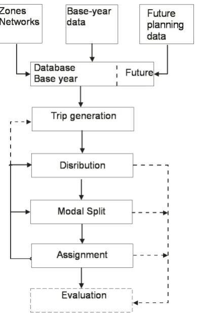
Figure 2.1: The classical transport model explained in section 2.3.

2.1

Transport models

Traffic managers are concerned with the optimiza-tion of road network performances, improving traf-fic conditions, reducing the congestion, and reduc-ing emissions. A traffic flow consists of different in-dividual drivers with their own inin-dividual behav-ior. Therefore traffic managers have to understand driver’s behavior. For understanding driver’s be-havior traffic managers use transport models. The transport models predict the deviation of the traffic flows over the road network [1]. Examples of trans-port models applications are: investigating the effect of changing a traffic light protocol on an intersec-tion, and predicting effects on traffic of development plans for a new Vinex location.

2.1.1

The classical transport model

Most transport models follow the structure of the classical transport model. The classical trans-port model is a four-step model [2]. The four steps of the classical model are: trip genera-tion, trip distribugenera-tion, modal split and the traf-fic assignment. The classical model is dis-played in figure 2.1. Next to the four steps, the figure displays feedback loops at the left side of the steps, these loops present iterations within the transport model. The steps and the feedback arrows are explained below with the use of an example. The example is printed italic.

(14)

14 CHAPTER 2. PROBLEM ANALYSIS

Figure 2.2: Plan of the example

Before starting the four steps, the network needs preparation. We divide the network into zones and collect, calibrate, and validate data about the zone and its inhabitants [2]. The number of zones depends on the re-quired level of detail of the model, and on the level of detail of the available data. Within a zone we specify only one centroid. A centroid is a location within the zone, which is the origin of trips from this zone and the destination of trips to this zone.

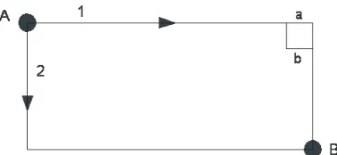
Village A and B are separated by a canal. A sketch of the environment of the villages is displayed in figure 2.2. At the south side of the villages a highway connects the two villages. The centers of the villages are connected with a rural road. The city councils of villages A and B want to know how many people will use the bridge on the rural road in 2020. To predict this amount the city councils provided results of a traffic research made in 2000. The city councils expect that village A will have 25% more inhabitants (from 200 to 250) in 2020 than in 2000, further they expect village B to keep the same amount of inhabitants (250 inhabitants). For simplicity of the example, we divide the network into four zones. In figure 2.3 the deviation into zones is shown, the dotted line represent the zone border. The circle in each zone represents the centroid. We define two zones outside the village A and B, to account for the traffic from outside the study area. We also number the links.

After the preparation of the network the first step, the trip generation starts. In the first step the attraction and production of traffic in each zone is determined. The production and attraction of trips is determined with socio-economic properties. For instance the number of households, or number of inhabitants in a zone for production, and the surface of office blocks, or number of full time employees for attraction. In general the production and attraction of trips with different purposes is identified separately. Often used trip purposes for modeling are: working trips, education trips, shopping trips, social and recreational trips and other trips [2].

The trip attraction and production in the year 2000 is shown in table 2.1, this is a result of the traffic research of 2000. We expect that every inhabitant of village A in 2020 will produce 3 trips and attracts 2 trips and that the inhabitants of village B in 2020 will produce 2 trips and attract 3 trips. Further, we assume centroid C and D produce and attract 100

(15)

2.1. TRANSPORT MODELS 15

(a) 2000

Zone Production Attraction

C 100 150

A 600 400

B 500 600

D 100 150

(b) 2020

Zone Production Attraction

C 100 100

A 750 500

B 500 750

[image:15.595.211.384.657.720.2]

D 100 100

Table 2.1: The production and attraction figures

trips. The attraction and production numbers for the year 2020 are given in table b of table 2.1.

In the second step (the distribution step) an Origin-Destination matrix (OD matrix) is developed. The number in cell (i,j) of the OD matrix is the amount of trips with origin i and destination j. The number of trips that start and end in each zone (calculated in the first step) are the row and column sums of the OD matrix. The inner cells of the OD matrix can be estimated with many different methods, for example growth factor methods or the gravity model. Growth factor methods can only be used if a base year OD matrix is available of the study area, because this method consists of multiplication on the old matrix. We use and explain the growth factor method in the example below. The gravity model takes into account the distance (or travel costs) between zones to determine the OD matrix. The gravity model can be written as: Tij = αOiDjf(cij). WhereTij is the number of trips from zone i to zone j,αa proportionality factor,Oi the amount of trips with origin i,Dj the amount of trips to destination j andf(cij)is a generalized function of the travel costs. The gravity model should be calibrated on a base year OD matrix, not necessarily of the study area [2].

(a) 2000

C A B D

C 0 30 70 0

A 100 100 350 50 B 50 250 100 100

D 0 20 80 0

(b) 2020

C A B D

C 0 31.39 68.65 0

A 71.5 149.55 490.64 38.55 B 28.5 298.00 111.73 61.45

D 0 21.07 78.99 0

Table 2.2: The OD matrices for 2000 and 2020

The OD matrix of the year 2000 is determined in the research of 2000, therefore we use the growth factor method. The OD matrix is given in table 2.2. The OD matrix for 2020 is calculated using the Furness method which is a growth factor method. Furness incorporates growth rates into new variablesaiandbj: Tij =tijaibjwheretij is the number of trips from i to j in the OD matrix of 2000 andTij is the estimated amount of trips from i to j for 2020. Furness proposes to fixbjwith value 1 first and find theaithat satisfies the amount of production found in the trip generation step. Next fix

aion the identified value and find the value ofbj that satisfies the amount of attracted trips found in the trip generation step. Repeat these proceedings until the changes are sufficiently small [2]. After six steps the OD matrix given in table 2.2 is found.

The trips of the OD matrix are made by different transport modes. A trip can be made for example by bike, by car, by train, or by bus. Therefore a third step, the modal split is needed, the trips are divided among the avail-able modes. Sometimes the modal split is simultaneously performed with the generation and distribution step.

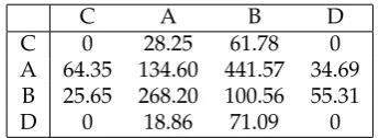
In the example 90% of all the trips are made by car, the others by bike. Our interest is only the car trips. The OD matrix for car trips is given in table 2.3.

C A B D

C 0 28.25 61.78 0

A 64.35 134.60 441.57 34.69 B 25.65 268.20 100.56 55.31

D 0 18.86 71.09 0

Table 2.3: The estimated car OD matrix of 2020

(16)

16 CHAPTER 2. PROBLEM ANALYSIS

[image:16.595.241.358.108.204.2]

In this research project, we focus on this assignment step, because we believe that the route choice results of a transport model are most influenced by the assignment step.

Figure 2.4: The process of the assignment step

We use a static assignment. The trips are assigned using an All or Nothing assignment, which means that the network loading is performed once and all the trips are assigned to the ’shortest’ path of their OD pair. The link costs are given in table 2.4, we used the link numbering of figure 2.3. We will explain the route choice between A and D. Travelers between A and D can take four different routes: on links 3-5-7, links 3-5-6-8, links 4-8, or links 4-6-7 (Traveling via zone C is obvious longer so routes via C will not be considered). The travel cost on these routes are respectively 63, 78, 72 and 69. Therefore the route 3-5-7 is the shortest route and is chosen. The total link flow on the bridge with the rural road between village A and B is 442+268=710, because travelers from A to B, and B to A choose a route with link 4.

1 2 3 4 5 6 7 8

22 15 8 40 32 6 23 32

Table 2.4: The link costs

After the assignment step the model is evaluated. If needed the model has to be adapted and calculated again. It is possible to adapt every step or even to adapt just one step. In every step, estimation errors are made and the results of every step should be validated and/or calibrated. However, if there is data available to calibrate or validate the model, the data usually consists of link counts. Route choice data or real OD matrices are very rare. The following example explains that even when there is link count data available calibrating on link counts will not ensure that the model is correct.

Consider our example study area. Suppose in 2020 we measure a link flow of 700 on the rural road bridge, which is close to the estimated 710 vehicles. In the model the 710 vehicles consists of travelers from A to B and B to A, but maybe the counted 700 vehicles consists of vehicles from zone A to B and A to D. In that case, our model does give proper link flows, but results in wrong traffic movements. Unfortunately, we do not notice the wrong traffic movements by calibrating on the link counts. Also we have to be aware of the measure errors incorporated in link counts.

2.1.2

Categories by the assignment step

The transport models are categorized by two different properties of the assignment step. One of these prop-erties is the scale of the assignment step. Transport models investigate traffic situations on three different assignment scales: macroscopic, mesoscopic, and microscopic. Macroscopic traffic flow research investigates the traffic flow in total on network level. Microscopic traffic flow research investigates the traffic flows at vehi-cle level, for instance the interaction between vehivehi-cles at corridor level [3]. Transport models with mesoscopic assignment steps operate between marcoscopic and microscopic models.

(17)

2.2. EQUILIBRIUM SITUATIONS 17

Figure 2.5: A town served by a bypass and a town center route

2.2

Equilibrium situations

In traffic research two special situations are often investigated: user equilibrium and social equilibrium. Traffic flows are stable in such situation. It is often tried to model an equilibrium situation because it is generally assumed that in normal conditions the reality approaches the user equilibrium, and because traffic managers want to realize the social equilibrium.

2.2.1

User equilibrium

Consider the town of figure 2.5. The road through the center has a capacity of 1000 vehicles per hour and the bypass has a capacity of 3000 vehicles per hour. Assume that during the morning peak 3500 vehicles per hour approach the town. Everyone would like the shortest route which is via the town center. It is clear that this road becomes congested when everyone chooses this road through the center. Many would opt for the bypass to avoid the long queues and delays. It is expected that drivers will vary their route on different days, until they find a more or less stable arrangement when none can decrease their travel time by switching to another route. This is a case of the user equilibrium, also called Wardrop’s equilibrium after his first principle. Wardrop’s first principle states: Under equilibrium conditions traffic arranges itself in congested networks such that all used routes between an O-D pair have equal and minimum costs while all unused routes have greater or equal costs [2] and [4]. This principle is based on the assumption that individual travelers are trying to minimize their travel costs.

2.2.2

Social equilibrium

The social equilibrium is based on Wardrop’s second principle. His second principle states:Under social equilib-rium conditions, traffic should be arranged in congested networks in such a way that the average travel cost is minimized. The social equilibrium is a target for traffic managers, who try to minimize travel costs. In principle traffic will not arrange itself according to the second principle, but the traffic will arrange itself following an approxima-tion to Wardrop’s first principle, the ’selfish’ or users’ equilibrium. To achieve a social equilibrium, travelers are assigned to links considering the marginal cost an additional traveler induces on link travel times [4].

2.3

Transport models used at DHV

DHV mainly uses three different computer programs as transport models: Questor, Dynasmart, and Aimsun. Questor is used for macroscopic static modeling, Dynasmart for mesoscopic dynamic modeling, and Aimsun for microscopic dynamic modeling. We believe that the assignment step of the transport model has the most influence on the route choice results, therefore we explain the assignment procedure of the three computer programs used by DHV.

2.3.1

Questor

(18)

18 CHAPTER 2. PROBLEM ANALYSIS

assignment iterations [6]. A fraction of the traffic is loaded on the network, the route costs are calculated and a smaller fraction is deloaded from the network. This process is repeated until the sum of the loaded minus the deloaded traffic is 100%. In the User Equilibrium assignment a fixed number of assignment iterations is used to approach the user equilibrium, at the end of each iteration step route costs are calculated. A fraction1−α

of the traffic is assigned according to the previous iteration step and a fraction ofαis assigned according to the new derived route costs. If equal weights are used in each iteration stepα(n+1) ₌ 1

n+1, than the Method

of Successive Averages (MSA) is obtained. A more efficient approach to reach the local minimum, the user equilibrium, is the Frank-Wolve algorithm. In the Stochastic User Equilibrium assignment, perceived travel costs instead of real travel cost are used. A random term is added to the link costs [5].

DHV works both with the Incremental and the User Equilibrium assignment. The Incremental assignment is a loading method. This loading method is used in combination with the shortest route principle in Questor.

2.3.2

Dynasmart

In Dynasmart travelers also follow their perception of the cheapest route or the k-cheapest routes. The percep-tion depends on the informapercep-tion available for the travelers. Dynasmart calculates the link costs on the basis of the travel times and toll costs. The user of the model defines the frequency of the route cost calculation. DHV chooses to calculate the cheapest route every simulation minute. A highway bias influences the link costs, to represent the preference for driving on highways. A highway bias of 0.15 is used to multiply the highway costs by 0.85. DHV uses a highway bias between 0.15 and 0.4. Two assignment procedures are possible in Dynasmart: One Shot assignment and Iterative Equilibrium assignment. In the One Shot assignment the trav-elers choose the shortest route on the basis of their perceived route costs and their behavior components. In the Iterative Equilibrium assignment the travelers are assigned to the network with the MSA. The MSA stops after a fixed number of iteration or when a preferred converge is reached.

In both assignment procedures Dynasmart assumes that the vehicles are fully informed about the link costs at the beginning of the trip. However not every traveler updates their calculation of the shortest route. Dynas-mart has five different user classes of vehicles. Three user classes are used in the One Shot assignment. Within these user classes the vehicles calculate the shortest route at the same instance. These user classes are:

• User class 1: These vehicles calculate the shortest route at the start of the trip. They follow this trip unless a VMSobligessomething else.

• User class 4: These vehicles calculate the shortest route at the start of the trip and every minute during their trip. Vehicles of user class 4 can change their route during a trip.

• User class 5: These vehicles calculate the shortest route at the start of the trip. They follow this route unless a VMSadvisessomething else.

User classes 2 and 3 are used at the iterative equilibrium assignment. User class 2 consists of travelers following routes according to the social equilibrium. Travelers of user class 3 follow the routes according to the user equilibrium. In the equilibrium assignment the traffic is a mix of user class 2 and 3 users, the fractions of the mix are defined by a parameter [7].

The Iterative Equilibrium assignment takes much more computation time than the One Shot assignment [8], therefore DHV mainly performs One Shot assignments.

2.3.3

Aimsun

Different from Dynasmart and Questor, the route choice model in Aimsun can use beside a user equilibrium also discrete choice models. Aimsun accounts cost for each link just like the other models. The link costs are based on travel time, the road capacity and sometimes a turning penalty (the Aimsun user chooses of which elements the link costs consist). First the initial costs with free flow speeds are calculated, except when there is a warm up period. In case of a warm up period, the initial cost are calculated at the end of the warm up period.

In the discrete route choice model assignment a simulation starts for a interval defined by the model user. In the simulation the travelers choose between the k-shortest routes and known predefined routes, with a route choice model. Aimsun has four different discrete route choice models: Multinomial logit, C-logit, Proportional method, and user defined route choice. In the user defined route choice the user defines the probability of use for known routes and the k-shortest routes. In the proportional method the route is proportional chosen to the route costs. The probability of choosing alternativeifor individualnin the proportional method is:

Pi =

CP_i−α

P

j∈KnCP

(19)

2.4. PROBLEMS 19

WhereCPjrepresents the route costs of routejandKnthe set of alternatives for individual n. The next chapter explains the Multinomial logit and the C-logit model. After assigning the predefined fraction, the cheapest paths are recalculated. Guided vehicles are provided with this new information and they are assigned to the new determined shortest route. Then the iteration starts again with simulating the next fraction of vehicles. Aimsun uses the Method of Successive Averages in the dynamic user equilibrium case. In the first iteration of the MSA the total amount of traffic is assigned to the cheapest route. After the first iteration, at iterationna fraction1/nis removed from the network and reassigned to a recalculated cheapest route. The algorithm stops after a fixed number of iterations or when the difference between the cheapest and the used routes is below a predefined acceptance gap (the user equilibrium is reached if the gap is zero) [9].

DHV uses the discrete choice assignment with the default settings of the C-logit route choice model. The default settings are used, because it is not know which settings leads to the most realistic results.

2.4

Problems

We notice two problems of the transport models at DHV. First the transport models often show travelers taking routes that we do not expect that travelers take in reality. Second the transport models are never calibrated or validated on the route choices, therefore we expect that unrealistic routing takes more often place than we observed. This section describes both problems.

2.4.1

Observed unrealistic routes

Observed unrealistic route choices seems to happen only in congestion situation in the three programs. Below three examples of observed unrealistic route choice are described.

Figure 2.6: Situation sketch of possible problem point for transport models

Consider the network in figure 2.6, the figure shows a highway with its on-ramp and off-ramp. Suppose congestion occurs at the highway. Travelers are directed to the shortest route at the start of their trip. During congestion on the highway, the shortest route could be: from the highway to the off-ramp, immediately to the on-ramp, and again to the highway (route 2). When many travelers are directed via the off- and on-ramp, congestion occurs at the off- and on-ramp. Travelers starting their trip when congestion occurs at the off- and on-ramp, are directed on the highway. It takes some time between the first travelers directed to the off- and on-ramp and the first time that congestion on the the off- and on-ramp. In this time all travelers are directed to route 2, a major fraction of them reach the off-ramp when congestion already occurred. The size of the congestion on the on-ramp will increase due to these travelers, while maybe the congestion on the highway is already disappeared. Route 2 is an unrealistic route from the moment congestion occurs at the off- and on-ramp. A similar problem occurs at a short parallel road between two sequential off-and on-ramps. Small adaptations to the model could solve this unrealistic routing. Traffic on the off-ramp can be prohibited to drive to the on-ramp. Unfortunately, sometimes it is possible to go left or right at the end of the off-ramp and turn near by and go to the on-ramp. In that case the interference makes the problem worse. This problem occurs in all transport model programs, but most often in Dynasmart. Dynasmart takes into account the blocking back effects of congestion (in contrast to Questor) and assigns all the traffic to one route in one assignment iteration (in contrast to Aimsun). Therefore, Dynasmart and Aimsun define more early another route as the cheapest than Questor. Dynasmart assigns more traffic at once to this route than Aimsun.

(20)

20 CHAPTER 2. PROBLEM ANALYSIS

zigzag through the network which seems very unrealistic.

A third problem occurs at Aimsun. The inner lanes of multiple lane-roundabouts are just a little bit shorter than the outer lane. Therefore travelers choose for the left lane and the right lane is not used. This behavior causes an unrealistic traffic situation.

2.4.2

Calibration and validation on route choices

We do not know to which extend the models used at DHV result in realistic route choices. DHV calibrates the transport model by adapting the OD matrix until the results will fit (within some boundaries) the traffic counts. As mentioned in section 2.1, the origin and destination of counted travelers are unknown. Calibrating on traffic counts will not ensure that counted travelers have the same origin and destination as the travelers in the model on these links have. Besides that, the results of the transport model depend on more steps than the trip distribution and errors can occur at every step (and at counting the traffic). We expect that improving one of the steps will lead to more realistic transport models. The route choice process has a major influence in the assignment step and is therefore an important aspect. DHV has never calibrated or validated the route choice model and we observe some unrealistic routing. Therefore we expect the biggest potential improvement of the transport model by improving the route choice process.

2.5

Conclusion

(21)

Chapter 3

Literature review

This chapter describes existing route choice models and approaches. Section 3.1 describes deterministic ran-dom utility based models, stochastic ranran-dom utility based models, and related issues of the ranran-dom utility based models. Section 3.2 describes other route choice models. In this master thesis project we investigate two of the described route choice models: the C-logit and game theory. Section 3.3 explains the choice for these two route choice models.

3.1

Random utility based models

The most common theoretical framework for generating discrete choice models is the random utility theory. In discrete choice models, travelers select from a finite set of alternatives, called a choice set [10]. The random utility theory is based on the following four properties:

• Individuals act rational, and are fully informed about the existence of links and their travel times.

• There is a setAof available alternatives, and a setXof vectors of measured attributes of the individuals and alternatives.

• Each alternativeihas associated a net utilityUinfor individualn. The modeler does not possess complete information about all the elements considered by the individual making the route choice decision. The modeler assumes that Uin can be represented by two parts, a deterministic and random part: Uin =

Vin+in.

• The individual selects the alternative with maximum utility [2].

In general the utility is expressed in a cost function, with travel time as the most important component. Ba-sically, the random utility based models can be divided into two groups: deterministic and stochastic route choice models. Deterministic route choice models always generate the same set of paths for an OD-pair. Most of the deterministic models can be made stochastic by using random generalized cost for the shortest path computations [11]. Stochastic methods generate an individual (or observation) specific subset. Stochastic route choice models based on the random utility theory are: Multinomial logit, C-logit, PS logit, Nested logit, and Cross Nested Logit.

3.1.1

Deterministic models

Deterministic route choice models assume that the travelers have full knowledge about the links and their ’costs’ in the network. A group of uniform travelers will therefore contribute the same link cost to a link according to deterministic route choice models.

Shortest Path

Most models of the deterministic group are based on the shortest path principle. In the shortest path principle, travelers are assumed to minimize on one variable or a mix of variables, for instance travel time or distance. At Questor a mix of travel times, toll costs, and distance expressed in costs is minimized. All travelers will choose the ’shortest’ route.

(22)

[image:22.595.203.392.55.142.2]

22 CHAPTER 3. LITERATURE REVIEW

Figure 3.1: Simple network with a path choice problem

Labeling approach

The labeling approach is another deterministic route choice model [11]. The labeling approach assumes that different travelers minimize different attributes. Some travelers may wish to minimize travel time, while other travelers feel uncomfortable driving on dangerous roads and avoid curvy roads. Each of these criteria may correspond to a different road being preferred, and thus, each route can be labeled with a different criterion for which it is the optimum. Examples of labels are: time, distance, fuel, scenery, traffic lights and congested travel. The labeling approach is used in combination with the Nested logit model when paths have multiple labels [4].

3.1.2

Stochastic models

Most stochastic route choice models are a member of the Generalized Extreme Value (GEV) family. GEV members described in this section are: Multinomial logit model, the C-logit, the Path Size logit, the Nested logit, and the Cross Nested logit. Mc Fadden derived the basic GEV model from the random utility theory [12]. The GEV model assumes that the random term in the utility function follows the Gumbel distribution. In the GEV models a choice set is defined. The choice setCn consists of all available alternative routes for individualn.

The Multinomial logit

The Multinomial logit model (MNL) is the most widely used choice model, due to its simple mathematical structure and ease of estimation [13]. According to the random utility theory the traveler choose his route from the choice set based on the net utilityUin. We as modelers do not have complete information about this net utility and try to describe the net utility by a deterministic partVinand a random partin. In the Multi-nomial logit is assumed that the random part can be described by the exponential Gumbel distribution. The probability of choosing alternativeifrom choice setCn in the multinomial logit model is therefore described by:

P(i|Cn) =

eθVin

P

j∈Cne

θVjn

Whereθis a scale parameter andVithe utility of routei. The utility of the routeVinis mostly expressed by the negative travel time, Section 3.1.3 discusses the utility expression in more detail. The exponential in the probability distribution ensures that large differences in travel times are highly recharged in the route choice probabilities.

A special property of the MNL is the Independent of Irrelevant Alternatives (IIA) property. Independent of Irrelevant Alternatives means that the ratio of the probabilities of any two alternatives is independent of other alternatives, so: P(i|C1)

P(j|C1) =

P(i|C2)

P(j|C2)[12]. First, this property was considered as an advantage of the model, due

to the property it is possible to forecast the share of a new alternative that is not present at the calibration stage if the attributes are known [2]. However this property has also a disadvantage, the disadvantage is explained below.

Someone is traveling from A to B in the network of figure 3.1. The travel times of route 1a, 1b and 2 are tminutes. Suppose that the utility is entirely based on travel time and that route 1b does not exist yet. According to the MNL the traveler will choose with probability et

2et = 0.5route 1a and with probability 0.5 route 2. Now the road b is finished and

(23)

3.1. RANDOM UTILITY BASED MODELS 23

The C-logit

The basic idea of the C-logit is to deal with similarities among overlapping paths (like route 1a and 1b in figure 3.1) through an additional "cost" attribute named commonality factor (CFi) [14]. Cascetta, Nuzzolo, Russo and Vitetta (1996) proposed the C-logit model, to maintain the computational simplicity of the logit form but produce more intuitive forecasts of route shares especially when path overlapping occurs. In contrary to the Multinomial logit consists the deterministic part of the net utility of two elementsVin−CFiinstead of oneVin. The probability that an individualnchooses routeiis formulated in the C-logit model by:

P(i|Cn) =

eθ(Vin−CFi)

P

j∈Cneθ(Vjn−CFj)

The scale factor, θ scales the effect that differences in systematic utilities (Vjn−CFj) have on the travelers decision, the largerθthe more influence of the differences. The commonality factor (CFi) of individualnfor routeiis proportional to the path overlap. Heavily overlapping paths have larger commonality factors and thus a smaller systematic utility with respect to similar, but independent paths. If pathiis made up of links belonging exclusively to that path, thenCFi is equal to zero [14]. In literature, we found five different forms of the commonality factor:

CFi = βln

X

j∈Cn

Lij

p

LiLj

!γ

(3.1)

CFi = βln

X

a∈Γi

la

Li

Na (3.2)

CFi = β

X

a∈Γi

la

Li

lnNa (3.3)

CFi = βln



1 + X

j∈Cn,j6=i

Lij

p

LiLj

Li−Lij

Lj−Lij



 [4] (3.4)

CFin = βln

X

a∈i

waiNa [14] (3.5)

Whereβandγare coefficients that weight the commonality factor,Lijis the common length of pathiand path

j,Γiis the set of arcs in pathi, andlathe length of linka.Nais the number of paths connecting the same OD pair which share linka, withNa = 1for centroid connectors [4], andwaiis the proportional weight of linka for pathi[14]. Formulation 3.5 is similar to formulation 3.2 ifwaiis chosen according to the distances. Larger values ofβcauses higher influence of the overlapping constant with respect to the utility. The influence ofγis smaller thanβand has the opposite effect. The parameterγis usually taken in the range [0,2] [9].

Formulation 3.1 is the only symmetric formulation. Symmetric means that the order in which routesiandj

are considered, does not influence the value of the commonality factor. In the other formulations, differences in route length will lead to an asymmetry [15].

In literature is not described which form of the commonality factor is the best formulation. There is a lack of theory or guidance to which form of commonality factor should be used [4]. Formulation 1 shows the most similarity with the Probit model, which we suspect to be realistic, but suffers from computational difficulties. Cascetta, Nuzzolo, Russo and Vitetta (1996) published the results of a calibration of the C-logit model with for-mulation 3.5. They calibrated the C-logit model for heavy truck route choice on the Italian national network. The calibration, with 1471 observations, shows that the usage of the commonality factor leads to significant improvements. They also found that the C-logit performs better when a limited number of alternatives with comparable path costs is considered [14]. Therefore, we advice to use the C-logit model in combination with a path generation algorithm which produces a limited number of such paths.

At DHV C-logit can be used in Aimsun. Formulation 3.1 is used in Aimsun. The default values in Aimsun are:

θ= 60,β= 0.15, andγ= 1. DHV uses always the default values, although it is not know if other values result in more realistic results.

Path Size logit

The Path Size logit (PS logit) also copes with overlapping paths. Like the C-logit, PS logit adds a correction term, the path sizeP S, to the utility function. The probability function is of the PS logit model is:

P(i|Cn) =

P SineVin

P

(24)

WhereP Sinis the size of pathifor individualn. Path-Size logit was introduced by Ben-Akiva and Ramming (1998), who presented the following formulation for the path size:

P Sin=

X

a∈Γi

la

Li

1

Nan

The term(la/Li)is a weight corresponding to the fraction of path impedance coming from a specific link. The termNais like at the C-logit the amount of paths using linka. This term is not affected by the length or impedance of the paths using it. Therefore, Ben-Akiva and Ramming ’s (1998) formulation of the correction term is not yet appropriate for long trips [4]. Ramming (2002) has developed a more general formulation:

P Sin=

X

a∈Γi

(la

Li

) 1

P

j∈Cn G(Li;γ)

G(Lj;γ)δaj

WhereGis a function with parameterγ. The value ofγrepresents the impact of the overlapping path lengths; the higherγthe more impact of the lengths [4]. Frejinger, Bierlaire and Ben-Akiva (2009) developed an ex-panded PS logit model. The route choice set is based on sample data in the exex-panded PS logit model. The Expanded PS shows good results and outperforms models with the original PS formulation [11].

The (Cross) Nested logit

The Nested logit (NL) is an extension of the MNL to deal with correlations between alternatives. The NL is most often used in mode choice and in multi-dimensional choice, such as combined destination and mode choice. Additional to the nested logit model the Cross Nested logit is developed. Nested logit models divide the choice setCn into m nests Cmn. The Cross Nested logit differs from the nested logit in that lower-level alternatives may belong to more than one nest [4]. The probability that individual nchooses alternative i

consists of two parts:

P(i|Cn) =P(Cmn|Cn)P(i|Cmn)

The choice probabilities of the Cross Nested logit are:

P(i|Cmn) =

αmieVin

P

j∈CmnαmjeVjn

P(Cmn|Cn) =

eVCmn+µmICmn

PM

l=1eVCln+µmICln

whereICmn =lnP_j_∈_Cmn(αmjeV jn)

1

µm _and_α_mi _{represents the membership of alternative}_i_{in nest}_m_{. The}

Cross Nested logit model is difficult to estimate because of the large number of nesting parameters [11], this reduces the usage of the Cross Nested logit. The Cross Nested logit is used for route choice modeling in small networks. We are unaware of applications of the Cross Nested logit in moderate size city [4].

The Probit model

The Probit model is not a member of the GEV family. The error terms in the Probit model follow a multivariate normal distribution. The Probit model incorporates the correlation among alternatives. Therefore, the Probit model uses a vector notation for the utility function:

Un=Vn+n

whereUn,Vn, andnare(Jn×1)vectors. The probability function of the Probit model is:

P(i|Cn) =P(Ujn−Uin≤0 ;∀j∈Cn) [12]

(25)

3.1. RANDOM UTILITY BASED MODELS 25

Mixed Logit models

Models with error terms distributed as a combination of normal and Gumbel distribution are: Mixed logit, Hybrid logit and Kernell logit. The general form of the Kernell logit model, in vector notation is given by Walker (2000):

U =Xβ+F T ξ+ν

WhereU is aJnby 1 vector of utilities,βis a column vector ofKunknown parameters;Xis aJnbyKmatrix of explanatory variables;ξis a column vector ofM i.i.d. standard Normal variables, which represent unob-servable factors;F is aJnbyM factor loading matrix;T is anM byM lower triangular matrix of unknown parameters; andνis aJnby 1 vector of i.i.d. Gumbel variables with scale parameterµ. The Logit Kernel model suffers from the same computational difficulties as pure Probit [4].

The Implicit Availability/Perception Logit Model

The Implicit Availability/Perception logit model (IAP logit) seems similar to the Multinomial logit model, but the IAP logit does not use a choice set. In fact the IAP logit starts with all existing alternative routes. IAP logit uses a correction term to a path’s share to reflect the possibility that travelers are unaware of that path, or unable to use it. The probability of using pathifor individualnis:

Pn(i) =

µn(i)eVi

P

j∈Mµn(i)eVi

WhereMis the set of all possible alternatives. We only know applications of the IAP logit with using variables related to availability and not with awareness. We expect that this route choice model will take too much computational time, because all existing alternative routes are considered.

3.1.3

Related Issues

Besides the parameters of the models, the utility function and the choice set major have influence on the route choice results of the random utility based models.

Utility function

It is clear that the deterministic utility termVinhas a major influence on the route choice results of the random utility based models. This term is often expressed by a combination of distance and travel time, because it is generally agreed that most travelers try to minimize travel time and distance for most types of journeys [16]. We also know that other elements like the amount of intersections, the amount of speed bumps, the view along the route, and the location of gas stations influence the route choice. The elements and the weights of the elements on which a route choice is based differ for every traveler. It is beyond the scope of this research project to investigate which elements and with which weights are the most realistic. We only consider different combinations of travel time and distance in the utility function. But we have to be aware that the route choice model could be improved by using other utility functions.

Choice set

(26)

3.2

Other Approaches

In the previous section we consider utility based models. This section discusses 4 other non utility based approaches. Non utility based models cope with the disadvantages of the random utility based models. Tver-sky and Kahneman (1986) have shown conflicts of the random utility theory with actual decision situation, therefore they developed the Prospect theory. Henn and Ottomanelli (2006) show that the consideration of randomness of traffic by drivers is hardly ever represented in random utility route choice models. These ran-domness of traffic by drivers is incorporated in Fuzzy logic. They also discuss that Possibility theory is more accurate in representing decision behavior under uncertainty than Probability theory which is used in the ran-dom utility theory. Game theory considers the traffic assignment from a totally different point of view. This theory considers the assignment as a game with multiple players. This section describes these four non utility based approaches and their applications in route choice modeling.

3.2.1

Prospect theory

Tversky and Kahneman (1979) developed the Prospect theory, because the random utility seems not to be the best theory to describe decision making. A first drawback is that the random utility theory is not developed from a psychological analysis of the decision making [18]. Second, the random utility theory does not take into account the certainty effect, the possibility effect, and the reflection effect. This lack causes conflicts of the random utility theory with actual decision processes. The example below shows the conflict with the cer-tainty effect. In the example, Kahneman and Tversky asked students to give their preferences on two problems.

Problem 1: Choose between

A: 2,500 with probability .33, B: 2,400 with certainty 2,400 with probability .66,

0 with probability .01; Problem 2: Choose between

C: 2,500 with probability .33, D: 2,400 with probability .34, 0 with probability .67; 0 with probability .66

The majority of the 72 respondents, 82% of the respondents preferred situation B against 18% for situation A in problem 2. In problem 2, 83% of the respondents choose C. Each of these preferences is significant at the 0.01 level. According to the random utility theory, withU(0) = 0, the first preference implies:

U(2,400) > 0.33U(2,500) + 0.66U(2,400)

0.34U(2,400) > 0.33U(2,500)

While the preferences of problem 2 implies the reverse inequality [19]. In the light of the previous and other observations from Kahneman and Tversky (1979), they argue that the random utility theory is not an adequate descriptive model. They propose the Prospect theory, which accounts for choice under risk.

Prospect theory distinguishes two phases in the choice process: editing and evaluation. Editing consists of the application of coding, combining, segregation and cancellation. Coding is the formulation of the offered prospects. Probabilities associated with identical outcomes are combined to simplify prospects. Segregation occurs to segregate risk less components from the risky component. Cancellation involves the discarding of common outcome probability pairs. In the evaluation phase the decision maker is assumed to evaluate each of the edited prospects, and to choose the prospect of the highest value. The overall value of a prospectV is expressed in two scales,πandv. the first scale,π, associates with each probabilitypa decision weightπ(p). The second scale,v, assigns to outcomexa numberv(x), which reflects the subjective value of that outcome. Hence,vmeasures the value of the deviations from the reference point. The value of prospect which is neither strictly positive nor strictly negative is formulated as:

V(c, p;y, q) =π(p)v(x) +π(q)v(y)

wherev(0) = 0,π(0) = 0, andπ(1) = 1. The evaluation of strictly positive and strictly negative prospect is different. These prospects are in the editing phase segregated in a risk less component and a risky component. Ifp+q= 1and eitherx > y >0orx < y <0, then:

V(x, p;y, q) =v(y) +π(p)[v(x)−v(y)]

(27)

3.2. OTHER APPROACHES 27

Figure 3.2: Hypothetical value and weighting function

Kahneman and Tversky (1979) proposed that the value function is defined on deviations from the reference point, generally concave for gains and commonly convex for losses, steeper for losses than for gains. Figure 3.2 displays a value function that satisfies these properties.

The weighting function is based on the overweighting property, subadditivity property, subcertainty prop-erty and subproportional propprop-erty. Low probabilities are generally overweighted, this mean thatπ(p) > p

for smallp, this is the overweighting property. The subadditivity property states that for small values ofp π(rp)> rπ(p)holds. Subcertainty entails thatπis regressive with respect top, preferences are generally less sensitive to variations of probability than you would expect. The subproportional property causes that the ra-tio of the corresponding decision weights is closer to unity when the probabilities are low than when they are high. This mean that if(x, p)is equivalent to(y, pq)then(x, pr)is not preferred to(y, pqr),0< p, q, r≤1. For example, suppose that a prospect of a gain of 40 with probability 0.5 is equal to a gain of 200 with probability 0.1, then the prospect a gain of 40 with probability 0.05 is not preferred to a prospect of 200 with probability 0.01. Figure 3.2 displays a weighting function that satisfies these four properties. The weighting function is not well-behaved near the end-points, because highly unlikely events are either ignored or overweighted, and the difference between high probability and certainty is either neglected or exaggerated.

Connors and Sumalee (2009) have successfully applied Cumulative Prospect theory on a two and a five link network. They used an equilibrium assignment, and derived the parameter values from choice modeling. Fur-ther research is needed to apply Prospect theory on real sized networks and to find meaningful parameters for the valuevand decision weightπfunctions [21]. Avineri and Prashker (2002) propose the Cumulative Prospect Theory Learning (CPTL) model, because the CPT static model failed to predict feedback based decisions. The CPTL is a dynamic generalization of the CPT model. The model uses travel time frequencies instead of travel time distributions, so instead ofpi the frequencyf rt(i)is used, for every time period t. They compare this model with three other models: Multinomial Logit model, the Cumulative Prospect Theory model, FL learn-ing model and the Reinforcement Learnlearn-ing model. The experimental results show that travelers’ behavior is better captured by learning models like the CPTL [22].

3.2.2

Fuzzy logic models

Henn and Ottomanelli (2006) show that the consideration of randomness of traffic by drivers is hardly ever represented in random utility route choice models. These randomness of traffic by drivers is incorporated in Fuzzy logic. Fuzzy logic is based on the concept of fuzzy sets. Fuzzy logic generalizes the notion of member-ship (to belong or not to belong to a set) to a continuous grade of membermember-ship (belonging more or less to a set). A fuzzy set is defined by its membership function,µawhich takes values in the interval [0,1]. In classical logic nothing can be concluded fromA⇒BifAis not observed, while in fuzzy logic a conclusion can be drawn if nearlyAis observed. Several route choice models using fuzzy logic are developed, with fuzzy linguistic rules such as "if travel time on route 1 is very short and travel time on route 2 is intermediate, then I will certainly choose route 1". In this linguistic rules are ’very short’ and ’intermediate’ fuzzy sets, which are based on expert knowledge.

(28)

28 CHAPTER 3. LITERATURE REVIEW

route choice model for multiple travelers, with the current knowledge and computation possibilities will take much computational time.

3.2.3

Possibility theory

Recently, researchers in psychology have begun to study the decision making behavior under uncertainty, and they have found that it seems that the possibility theory is more close to the mental framework than the probability theory. Therefore possibility theory seems a promising theory for route choice modeling. The possibility theory is developed as an alternative way to probability in order to represent uncertainty. While probability is based on the additivity axiom, possibility is based on some max-axiom: Given two subsetsA

andBin the universeX, the probability and possibility measures are:

P r(X) = 1 P oss(X) = 1, P r() = 0 P oss() = 0,

P r(A∪B) =P r(A) +P r(B)−P r(A∩B), P oss(A∪B) = max{P oss(A);P oss(B)}.

The probability that travelernchooses alternativeiis supposed to be proportional to the possibility that a cost is smaller or equal to others. Applying the normality condition for probability, we get:

Pn(i) =

P oss(Ce_in<Ce_jn∀j6=i) P

iP oss(Ce_in <Ce_jn∀j6=i)

A few fuzzy based route choice model already use the possibility theory [1]. Like in the case of Fuzzy logic based models, we expect that possibility theory route choice models will take much computational time.

3.2.4

Game theory

Game theory is a mathematical theory to analyze situations with competition and cooperation between several parties. This is a broad definition of game theory, but is in consensus with the broad spectrum of applications of game theory. The applications range from strategic questions in warfare to understanding economic com-petition, and also include traffic situation. The problems of these applications are displayed as a game. The decision makers of the application are the players in the game. The players of the game can make a move, which we call an action. The result of the game is the final payoff, which is the optimal gain if every player plays his optimal strategy [23]. The game will reach an equilibrium situation if every player plays according to their optimal strategy.

Two travelers use the network of figure 3.3, a tractor and a car. Both travelers are going to the gas station, the tractor favors the northern route and the car the southern route. The tractor arrives first at the network and decides if he takes the northern route or the southern. The car arrives later and cannot see which route the tractor has taken. If the car takes the same route as the tractor, the car will be delayed due to the slower tractor, and the tractor will get nervous of the car behind him. The southern route is the most smallest route and they will bother each other the most on this route. The gain for each decision situation is displayed in table 3.1, the tractor chooses a row and the car a column. We translate this situation into a two player non cooperative game. The players are the tractor and the car, both want to maximize their gain (utility). By choosing the northern route the tractor is always at least as well off as by choosing the southern route. So the optimal strategy of the tractor is choosing the northern route. The car, being able to perform this same kind of reasoning for the prediction of the action of the tractor, has the southern route as optimal strategy. Since the southern route is the best reply to the choice of the northern route by the tractor.

(29)

3.2. OTHER APPROACHES 29

northern route southern route

northern route 4 5

southern route 4 1

Table 3.1: Gain of the decision situations

The previous example is a very simple traffic situation with only two travelers and a small network. But this example can easily be extended to a more complex network with more (even infinite) travelers. Often, the so-lutions are not that straight forward as in the example. The optimal strategy of the example is a pure strategy. In pure strategies, players choose always exactly one route; the tractor always chooses the northern route and the car always chooses the southern route. In mixed strategies, players choose with a probability distribution overmparallel routes in a mixed strategy.

Congestion game

In literature several different games with applications in traffic situation are described. The n-player conges-tion game is the most simple game described. A congesconges-tion game is a non cooperative game, meaning that players cannot make agreements with each other [23]. The payoff of the players depends only on the player ’s own strategy and on the number of other players choosing the same or some interfering strategy. A player represents one vehicle of the network.

We describe the congestion game with travel times as negative payoff by the following mathematical model. LetP ={1, ..., N}denote the set of players. Each playeri∈Pmaximizes its own payoff, they minimize their expected travel time.

min X

j∈Ai

(T Tj(x)·si(j))

whereAiis the action set of which playeriselects an action (a route),T Tj(x)the travel time of routejwith loadingx,sithe mixed strategy of playeri, andsi(j)the probability that playerichooses routejaccording to his strategy. The travel time of routejconsists of the sum of all link travel times of routej:

T Tj(x) = L

X

l=1

[image:29.595.295.514.467.740.2]

(LT Tl(x(l))·P L(j, l))

Figure 3.4: The process of the congestion game whereLis the total amount of links in the

net-work,LT Tl(x(l))the travel time of linkl with loadingx(l)on linkl, andP L(j, l) = 1if linkl

is an element of pathjotherwiseP L(j, l) = 0. The amount of traffic on the links is calculated by:

x(l) =X

i∈P

X

j∈J

(si(j)·P L(j, l))

The mixed strategysiis conditioned by two re-straints:

X

j∈J

si(j) = 1 and si(j)≥0

(30)

30 CHAPTER 3. LITERATURE REVIEW

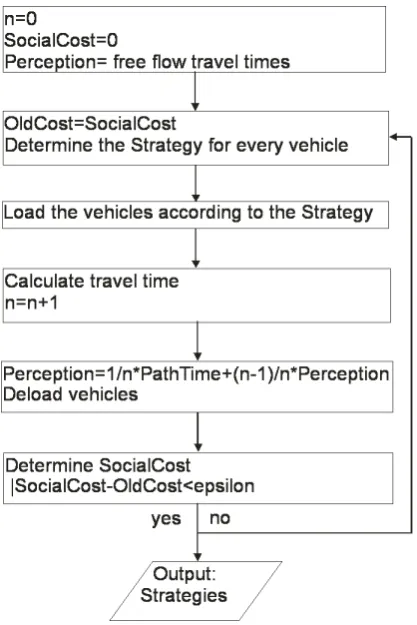
path times:SC=PL

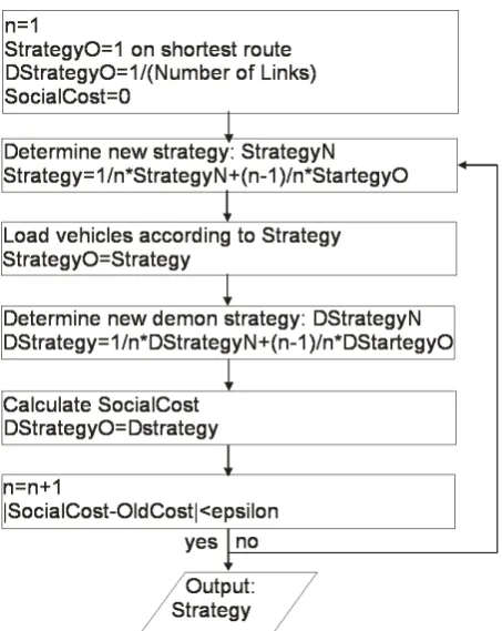
l=1LT Tl·x(l)withLthe amount of links, andLT Tlthe travel time of linkl. This process is repeated until the differences between the SocialCost and the OldCost is within some predefined bounds. The output of this iterative scheme is the mixed strategy of the players to reach the flow of the final iteration. Players of the same origin destination pair will have the same optimal mixed strategy.

The congestion game always reaches a Nash equilibrium of pure strategies. The process of the congestion game will always converge [24].

Smooth fictitious play

Garcia, Reaume & Smith (2000), Cominetti, Melo & Sorin (2008) use the perception of travel times instead of real travel times to model traffic routing. Both use a fictitious play to incorporate a learning effect in the perception of travel times. Fictitious play is an iterative procedure in which at each step, players compute their best replies based on the assumption that the opponents’ decisions follow a probability distribution in agreement with the historical frequency of their past decision [25]. Garcia et. al. (2000) describe the results of Monderer and Shapley (1996) who demonstrate that fictitious play convergences in some sense, when players share a common objective function. Therefore, Garcia et. al. (2000) assign the players with a common objective function instead of a selfish. The player’s objective is to minimize average trip time of all travelers. This game is called the Fictitious Dynamic Traffic Game [25]. In reality people do not act that socially, people rather want to minimize their own travel time than the average travel times of all vehicles. Cominetti et. al. (2008) base their model on this thought, assuming that the travel times of other vehicles are unknown. Their iterative fictitious play is based on the vehicles own travel times, and is called the smooth fictitious play.

[image:30.595.59.268.400.713.2]

The game of the smooth fictitious play is iteratively played, each stage can be described by the same mathe-matical model. Therefore we describe just a single stage. Again letP ={1, ..., N}denote the set of players. Each playeri∈Pmaximizes their own payoff, the negative perception of their travel time under the assump-tion that the other players play the acassump-tion (the routes) whose probability distribuassump-tion is given by historical frequency’s of past plays [26].

Figure 3.5: The smooth fictitious play

minX

j∈Ai

(P T T_in(j)·sn_i