Graph theoretical aspects of constraint solving in the SST project

(1)

Master’s thesis

Graph-theoretical aspects of constraint

solving in the SST project

by Jacob J. Koelewijn

Supervisors: Dr. Georg J. Still Prof.dr. Marc J. Uetz Ir. Matthijs J. Bomhoff

(2)

Acknowledgements

This thesis is the result of my work for the Final Project of my master’s degree program in Applied Mathematics at the University of Twente. First of all I’d like to say thanks to Georg Still, my main supervisor. Without his help this thesis wouldn’t be possible. He guided me through the process and assisted me where necessary, both during the research itself and the writing of this thesis.

Also thanks to Matthijs Bomhoff, who was my main adviser. He made very useful remarks about my work during discussions. Thanks to Marc Uetz, for taking part in my graduation committee.

(3)

1

Introduction

This thesis covers some graph-theoretical aspects of constraint solving in theSmart Synthesis Tools project(SST project). So let’s begin with a small in-troduction of the project and the problems that will be of interest for this thesis. A more general overview of the SST project can be found in Ap-pendix A.

The aim of the SST project is to develop software with the ability to gener-ate and analyze a number of different designs of a product or a machine. The constraint solving part of this software involves solving large under-constrained systems of equations. This problem is analyzed by construct-ing a bipartite graph associated to the structure of the system of equations. This will be discussed in Chapter 2.

Different decompositions of the bipartite graph and their use for solving the system of equations are investigated in Chapter 3. Also, properties of the decompositions are proved in a new way in terms of maximum match-ings. In Chapter 4, the Quasi-Newton method and its use for the SST project will be described, namely to find solutions of the subsystems that are found using the decompositions.

Besides the decompositions, the bandwidth reduction problem for unsym-metric matrices is investigated in Chapter 5. A reduction of bandwidth allows for more efficient storage and calculation when solving big sparse systems of linear equations using banded algorithms. Also in this case, the problem will be approached by looking at a bipartite graph corresponding to a problem instance.

(6)

2

Structure of systems of equations

2.1 Introduction

Let us call the the software that is being developed for the SST project the SST framework. One important goal of the SST framework is to generate a number of (different) designs of a product or machine given amodelwhich contains certain properties and constraints. Such a model consists of param-etersandrules. Actually, in the SST framework, the parameters and rules are ordered within a tree to provide different abstraction levels, but this is outside the scope of this thesis.

Theparametersof the model describe the properties of the final design, such as width, height, location of certain components, material, etc. A specific assignment of values to the parameters correspond to a unique design. To be able to analyze them, all parameters in this thesis will be real variables. Therulesof the model describe the constraints for the final design, such as a minimal and maximal width, a specific distance between two components, a direct relation between parameters, etc. In a feasible design, all rules must be satisfied. For the sake of analysis, all rules in this thesis will be (nonlin-ear) equations. They will be implemented as nonlinear functions of the parameters that should evaluate to zero for a valid design/solution. Re-quirements of the SST project dictate that the functions have a “black box” property, i.e. no analytical information about the functions is available. The only information that is available to the SST framework is which parame-ters are explicitly present in a rule and the evaluation of a rule-function given the values of its dependent parameters.

(7)

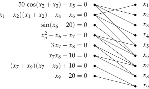
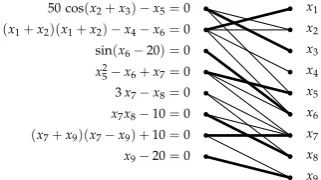
50 cos(x2+x3)−x5 =0 (x1+x2)(x1+x2)−x4−x6 =0

sin(x6−20) =0

x2₅−x6+x7 =0

3x7−x8 =0

x7x8−10=0 (x7+x9)(x7−x9) +10=0

x9−20=0

x2

x1

x3

x4

x5

x6

x7

x8

[image:7.595.180.437.127.280.2]

x9

Figure 2.1: An example of a system of equations with it’s associated bipar-tite graph

Chapter 3 can be found in Section 2.3 and Section 2.4 will give an introduc-tion into the generaintroduc-tion of a feasible design using an interactive solver.

2.2 Notation and definitions

2.2.1 Problem instance

We are working with a problem instance that can be defined as follows. Let h :Rn_→_Rp_{. Then}_h₍_x_{) =}_{0 represents a system of}_p_{(nonlinear) equations.}

Because of the nature of the smart synthesis problems this system will most likely be under-constrained, i.e.p< n. Let

hl(x) =0, l∈ L={1, . . . , p}

be the equations of this system. pis the number of equations and xis the vector of variables xi with i ∈ I = {1, . . . , n}where n is the number of

variables.

We can construct a bipartite graph associated to this system. LetG= (V,E)

be this bipartite graph with vertex setV = L∪I and edge setE ⊆ L×I. Land I are the vertex classes of the bipartite graph. There is an edgee = (`,i)_∈ Eiffh`(x)depends explicitly onxi.

(8)

2.2.2 Definitions

Sets

Asetis a unordered collection of distinct objects. An object in a set is called anelementof the set. LetAandBbe two sets. Theunion A_∪Bis the set of all elements that are an element of eitherAorB. Theintersection A∩Bis the set of all elements that are an element of both AandB. IfA∩B= ∅, then

AandBare said to bedisjoint. Thedifference A\B, is the set of all elements that are an element of Abut not of B. Note that not all elements ofBhave to be in A. The symmetric difference A₄Bis the set(A_∪B)_\(A_∩B). In

other words, the symmetric difference is the set of elements that are inAor inBbut not in both. The cardinality_|S_|of a setSis the number of elements ofS.

Graphs

Asimple graph(or justgraph) G= (V,E)consists of a setVof vertices and a setEof edges. Anedgeis an unordered pair of distinct vertices ofV. Two different vertices v1,v2 ∈ V are called adjacentwhen there exists an edge (v1,v2) ∈ E. Two different edges are called adjacent when they share at

least one vertex. Awalk is a sequence of consecutive (adjacent) edges. A pathis a walk with distinct edges where every vertex is traversed at most one time. Atouris a walk in which the first and last vertices are the same. A cycleis a path in which the first and last vertices are the same. Two vertices v1 and v2 are connected when there exists a path in which the first vertex

isv1and the last vertex isv2. A graph G0 = (V0,E0)whereV0 is a subset

ofVandE0 _{is a subset of}_E_{containing only pairs of vertices in}_V0 _{is called}

a subgraph of G. For a set of vertices X ⊆ V, we useG[X] to denote the

induced subgraphofGwith vertex setXand with edge setE_∩(X_×X). In

words: the edge set ofG[X]is the subset ofEconsisting of those edges with both ends inX.

Adirected graph G= (V,A)consists of an collectionVof vertices and a

col-lection Aof arcs. Anarcis an ordered pair of distinct vertices ofV. An arc

(9)

a walk formv1tov2and a walk fromv2andv1. Thestrongly connected

com-ponentsof a directed graph are the maximal strongly connected subgraphs. For a set of verticesX _⊆V, we useG[X]to denote theinduced subgraphof

Gwith vertex setXand with arc setA∩(X×X).

Abipartite graph G = (V,E)is a graph that has two vertex classesLand I

such thatL_∪I =VandL_∩I =∅. Avertex classofGis a vertex setL_⊆V

with the property that there is no edge(`₁,`₂)inEwith`₁,`₂_∈ L.

For ease of notation consider a set operation between a graphG = (V,E)

and an edge setE0_{as an operation between}_E_and_E0_{, i.e.}_G_∩_E0 _{can be read}

as E∩E0_{. Similarly consider a set operation between a graph} _G _{= (}_V,_E₎

and an vertex setV0_{as an operation between}_V_and_V0_{. In case of ambiguity}

E(G)will be used to denote the edge set EofGandV(G)will be used to denote the vertex setVofG.

Matchings

Given a bipartite graphGas defined in Section 2.2.1, amatchingforGis a subset M ⊆ Esuch that every vertex ofGis incident to at most one edge of M. Amaximal matching of a bipartite graphG is a matching M that is not a proper subset of any other matching in G. A maximum matching of a bipartite graphGis a matching Mwith the property that there exists no other matching M0 _of _G_with _|_M0_| _> _|_M_|_{. A matching} _{M covers}_{a vertex}

v1 ∈ Vwhen there exists a vertexv2 ∈ V with (v1,v2) ∈ M. A matching

M coversa set of verticesV0 _⊆_V_when_M_{covers all vertices in}_V0_{. A}_perfect

matchingof a bipartite graphGis a matchingM with the property thatM coversV. Note that this is only possible when|L|=_|I|.

2.3 Consistency concept

To give an idea of consistency consider the following three systems of equa-tions:

(2.1)

x1+x2 =2 x1

(10)

(2.2)

x1+x2 =2 x1

x2

x1+2x2 =1

(2.3)

x1+x2 =2 x1

x2

x1+2x2 =1

x1+3x2 =4

System (2.1) has an infinite number of solutions. For every value ofx1there

is a valuex2 = 2−x1that makes the equation sound. In this system there

is one equation and there are two variables.

System (2.2) has exactly one solution (x1 = 3, x2 = −1). The system has

two equations and two variables.

System (2.3) has no solution at all. The reason for this is that the first two equations only allowx1andx2to have values 3 and −1 respectively. The

third equation contradicts to this.

Most of the time a system of equations does not have a solution when it has more equations than variables. Moreover, when a subsystem has more equations than variables, the whole system has no solution most of the time. This is a situation we want to avoid. We need a definition.

Definition 2.1. LetG = (V,E), withV = L∪I, be a bipartite graph. For a subsetL0 ⊆ L, theneighbor set N(L0)⊆ I is the set of nodes in I that are

adjacent to at least one node inL0.

Definition 2.2. A system of equations and its corresponding bipartite graph are called (structurally)consistentwhen the following holds:

|N(L0)| ≥ |L0| ∀L0⊆ L. (2.4)

When a system is consistent, a situation like (2.3) is automatically avoided. There is another criterium for consistency.

Corollary 2.3. A system of equations is (structurally) consistent iff its associated bipartite graph contains a (maximum) matching covering L.

(11)

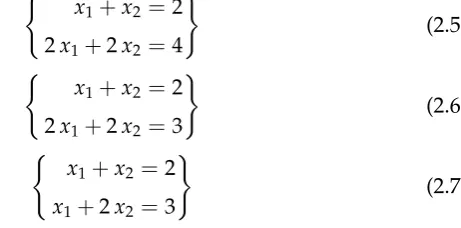
h1(x) x1

x2

[image:11.595.249.480.570.684.2]

h2(x)

Figure 2.2: Bipartite graph corresponding to the Systems 2.5, 2.6 and 2.7

Note that for a system of equations where the number of equations is the same as the number of variables, as a consequence of Corollary (2.3), con-sistency implies that its associated bipartite graph contains a perfect match-ing.

Let us call a systemhof equationsh`(x) =0 (structurally)under-constrained

when its associated bipartite graph has a maximum matching covering all nodes of L and|L| < _|I_|, i.e. there are more variables than equations. A

systemh of equationsh`(x) = 0 is (structurally)over-constrainedwhen its

associated bipartite graph has a maximum matching covering all nodes of I and_|L_| > _|I_|, i.e. there are more equations than variables. A system h

of equationsh`(x) = 0 is (structurally)well-constrainedwhen its associated

bipartite graph has a perfect matching. A bipartite graph is called under-, over- or well-constrained when its associated system is respectively under-, over- or well-constrained.

2.3.1 Limitations and possibilities

Let’s have a look at the limitations of analyzing a system of equation using the structure of its associated bipartite graph. As Ait-Aoudia et al. (1993) pointed out there is no one-to-one relation between a bipartite graph and the fact whether the corresponding system can be solved. For example the systems

(

x1+x2 =2

2x1+2x2 =4

)

(2.5)

(

x1+x2 =2

2x1+2x2 =3

)

(2.6) (

x1+x2=2

x1+2x2=3

)

(2.7)

(12)

so-lutions, System (2.6) has no solutions at all and System (2.7) has just one solution. The reason for this is that the Jacobian matrix Jh of Systems (2.5)

and (2.6) is singular.

This simple example shows clearly that it is not possible to say something about the solution space of a specific system of equations by analyzing its corresponding bipartite graph (structure).

However, it is possible to say something about the class of systems of equa-tions that are consistent. This problem has been more thoroughly investi-gated by Still et al. (2010). Some of the main results of this work will be summarized in the remainder of this subsection without proof.

Let us consider a system of nonlinear equationsh: Rn _→_Rn_with_n

equa-tions and n variables and its associated bipartite graph G = (V,E) with V =L∪I. It is well-known that for any solution ¯xofh(x) =0 the Newton

iterationx_k+1 = xk−[Jh(xk)]−1h(xk)is locally quadratically convergent to

¯

xif the regularity condition holds:

Jh(x¯) is nonsingular . (2.8)

Callh regularwhen (2.8) holds for all solutions ¯xof h(x¯) = 0 andirregular

otherwise.

Corresponding to the bipartite graphG= (V,E)withV= L_∪I we define

the function setSG,

SG =

n

h :Rn→Rn,h∈C1|hi depends onxjonly if (i,j)∈E

o

where SG ⊂ C1(Rn,Rn)is endowed with the so-called strong topology as

defined in Jongen et al. (2000). Theorem 2.4. When G is consistent,

(a) and h∈SGis regular, any (sufficiently) small perturbationh˜ ∈SGof h will

result in a regular functionh.˜

(b) and h _∈SGis irregular, by an arbitrarily small perturbation a regular

func-tionh˜ ∈SGcan be obtained.

When G is not consistent,

(c) h ∈SGis irregular. Even more, every solutionx of h¯ (x¯) =0will not satisfy

(13)

SST framework

Interactive solver

Analysis

[image:13.595.185.427.129.222.2]

Partial solver

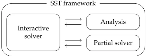
Figure 2.3: Schematic overview of interaction of the solver

(d) and h∈ SG, any (sufficiently) small perturbation of h will result in a

func-tionh˜ ∈SGsuch thath˜(x¯) =0has no solution.

So to be able to solve h with a Newton method, it is important that Gis consistent. Note that Systems (2.5) and (2.6) can be made regular by chang-ing one of their coefficients by a arbitrarily small value e 6= 0, resulting

in systems with just one solution. Also note that for nonlinear systems of equations, consistency does not guarantee the existence of a solution.

2.4 Interactive solver

Parallel to the investigation of the structure of the system of equations, the application to the interactive solver of the SST project will be discussed. Theinteractive solveris a part of the SST framework that generates one fea-sible design (solution) given a model (system of equations) as input. It will also be referred to as thesolver. One of the requirements of the solver is that when it generates different feasible solutions, these solutions should be as different from each other as possible, i.e. they should be a good represen-tation of the total solution space.

Theinputof the interactive solver is an (underdetermined) system of equa-tions and its associated bipartite graph. Theuseris the decision maker that controls the interactive solver. In this thesis, the SST framework is the user, i.e. the solving process will run automatically.

(14)

(15)

3

Dulmage-Mendelsohn

decompo-sition

There exists a unique decomposition of a bipartite graph that splits the graph in an under-, over- and well-constrained part. This decomposition was first described by Dulmage and Mendelsohn (1958, 1959, 1967). Their decomposition also decomposes the well-constrained part into irreducible components. Several authors distinguished between the two levels of the decomposition: just like Pothen (1984) this work will use the term coarse decomposition for decomposition in an under-, over- and well-constrained part and fine decompositionfor the decomposition of the well-constrained part. It may be noted that the terminology of this work differs from that of Dulmage and Mendelsohn (1958, 1959, 1967) and is more similar to Pothen (1984) and Lovász and Plummer (1986).

The main goal of Subsections 3.1 and 3.2 is to provide a proof of the de-composition of Dulmage and Mendelsohn in terms of maximum match-ings. This exact way of proving the Dulmage-Mendelsohn decomposition is new. However, the proof contains elements of the proofs of Pothen (1984) and Lovász and Plummer (1986).

3.1 The coarse decomposition

Lovász and Plummer (1986) give the following definition of the coarse de-composition.

Definition 3.1. The coarse decomposition of a bipartite graph G = (V,E)

with V = L∪ I (see Section 2.2.1) consists of three disjoint vertex setsV1,

V2, andV3. Let D⊆ Vbe the set of all vertices ofGfor which there exists

(16)

AI

CL CI

50 cos(x2+x3)−x5=0 (x1+x2)(x1+x2)−x4−x6=0

sin(x6−20) =0

x2

5−x6+x7=0

3x7−x8=0

x7x8−10=0 (x7+x9)(x7−x9) +10=0

x9−20=0

x2

x1

x3

x4

x5

x6

x7

x8

x9

DL

DI

AL

V3

V1

[image:16.595.152.458.118.323.2]

V2

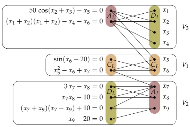
Figure 3.1: The groupsV1,V2andV3

A ⊆V−Dbe the set of all vertices outsideDthat are adjacent to a vertex in D. And letC = V−D−Abe the set of remaining vertices. Now split the sets according to the bipartition ofG, i.e.AL= A∩L,AI = A∩I,CL =

C_∩L,CI = C∩I, DL = D∩LandDI = D∩I. Finally letV1 = CL∪CI,

V2 =DL∪AI andV3 = AL∪DI (as in Figure 3.1).

The coarse decomposition has some useful properties that will be stated in the next theorem.

Theorem 3.2. The coarse decomposition satisfies the following conditions. (a) The decomposition is unique.

(b) The are no connections between CL and DI and there are no connections

between CIand DL.

(c) There are no connections between DLand DI.

(d) The system corresponding to V1is well-constrained, the system of V2is

over-constrained and the system of V3is under-constrained.

To prove Theorem 3.2 more work is needed. See the next subsection.

Proof of Theorem 3.2

(17)

50 cos(x2+x3)−x5=0 (x1+x2)(x1+x2)−x4−x6=0 sin(x6−20) =0 x2

5−x6+x7=0 3x7−x8=0

x7x8−10=0 (x7+x9)(x7−x9) +10=0 x9−20=0

x2 x1 x3 x4 x5 x6 x7 x8 x9

(a) The matching M1 consisting of the thick lines

50 cos(x2+x3)−x5=0 (x1+x2)(x1+x2)−x4−x6=0 sin(x6−20) =0 x2

5−x6+x7=0 3x7−x8=0

x7x8−10=0 (x7+x9)(x7−x9) +10=0 x9−20=0

x2 x1 x3 x4 x5 x6 x7 x8 x9

(b) The matching M2 consisting of the thick lines

50 cos(x2+x3)−x5=0

(x1+x2)(x1+x2)−x4−x6=0 sin(x6−20) =0 x2

5−x6+x7=0 3x7−x8=0

x7x8−10=0

(x7+x9)(x7−x9) +10=0

x9−20=0

x2 x1 x3 x4 x5 x6 x7 x8 x9

[image:17.595.318.479.137.227.2]

(c) The symmetric differenceM14M2

Figure 3.2: An example of a symmetric difference

computation of the coarse decomposition.

For (a) observe that the sets are well-defined thus the decomposition is unique for a specific bipartite graph. (b) follows directly from Definition 3.1. We are going to analyze which vertices are in DL and DI. It is obvious

that the vertices in Lnot covered by Mare in DL and the vertices inI not

covered byMare inDI. We need an auxiliary lemma.

Lemma 3.3. The following equivalences hold for vertices in DLand DI.

(a) A vertex uL ∈ L is in DL ⇐⇒ uLis reachable by an M-alternating path

starting from a vertex in L not covered by M. Clearly, this path must have an even length (zero length is also possible).

(b) A vertex uI ∈ I is in DI ⇐⇒ uI is reachable by an M-alternating path

starting from a vertex in I not covered by M. Clearly, this path must have an even length (zero length is also possible).

Proof. Only (a) will be proven, the proof of (b) is similar by symmetry.

(18)

⇒Suppose there is a vertexuL∈ DLthat is covered byM. Then there exists

(by definition ofD) a maximum matchingM0_where_u_L_{is not covered. Now}

take the symmetric differenceSofMandM0_{(see Figure 3.2 for an example}

withuLcorresponding to 3x7−x8). Because each matching can contribute

maximum 1 degree to a vertex inSthe symmetric difference consists only of cycles and paths. The paths are of even length because both matchings are maximum (since an odd length path would result in an augmenting path in eitherMorM0_{). Because}_u_L_{is only covered by}_M,_u_L_{is an end-vertex of}

a pathPin the symmetric differenceS. Pis anM-alternating path of even length so the other end-vertex of path P must be a vertex not covered by M.

Now (c) can be proven.

Proof of (c). Suppose there is an edge(uL,uI)with uL ∈ DL anduI ∈ DI.

Then by Lemma 3.3 there exists an M-alternating pathP1starting in a

ver-tex inLnot covered byMtouL. By symmetry there exists anM-alternating

path P2 starting in a vertex in I not covered by M to uI. If (uL,uI) ∈/ M

then combining P1, (uL,uI) and P2 results in an augmenting path for M,

which is a contradiction becauseMis maximum. Notice that there can’t be an edgee that is in bothP1andP2because otherwise it would be possible

to construct an augmenting path forM, which is a contradiction.

So let’s consider the case that(uL,uI) ∈ M. We know there exists an

M-alternating path P starting in a vertex in L not covered by M to uL. The

last edge of theM-alternating path must be inMbecause the first (starting) edge of P is not in M and P has even length. This means that (uL,uI)

must the last edge ofP, because otherwise(uL,uI)can’t be in M, which is

a contradiction. By the same argument there exists an M-alternating path P0 _{starting in a vertex in}_I_{not covered by}_M_to_u_I_{where the last edge of}_P0

is(uL,uI). But now combining the M-alternating paths PandP0\(uL,uI)

results in an augmenting path forM, which is a contradiction becauseMis maximum.

Before proving (d) we need two other auxiliary lemmas.

(19)

(a) A vertex uI ∈ I is in AI ⇐⇒ uI is reachable by an M-alternating path

starting from a vertex in L not covered by M. Clearly, this path must have an odd length.

(b) A vertex uL ∈ L is in AL ⇐⇒ uLis reachable by an M-alternating path

starting from a vertex in I not covered by M. Clearly, this path must have an odd length.

Proof. We’ll only prove (a), the proof of (b) is similar by symmetry.

⇐LetvLbe the vertex beforeuIin theM-alternating path. By Lemma 3.3

we know thatvLis inDL. ObviouslyuIis adjacent tovLsouIis inA(by (c)

uLcannot be inDI). BecauseGis bipartite we knowuI is inAI.

⇒ Because uI ∈ AI there exists a vertex vL ∈ DL adjacent to uI. By

Lemma 3.3 it is known that there exists an M-alternating path P from a vertex in Lnot covered by matching M to vertex vL of even length. If P

goes through uI we are done. So suppose thatP does not go throughuI.

Note that in this casevLcan’t be matched touI byMbecause the last edge

of Pmust be a matching edge. Now P∪(vL,uI)is an M-alternating path

of odd length.

Lemma 3.5. For an edge(`,i) _∈ M with i _∈ AI it is always true that` ∈ DL.

And for an edge(`,i)∈ M with`_∈ A_Lit is always true that i_∈ D_I.

Proof. Only the first statement first will be proven, the second statement is true by symmetry. Lemma 3.4 tells us that there exists an M-alternating pathPstarting in a vertex inLnot covered byMtoi.Phas odd length and its first edge is not inM because the starting vertex ofPis not covered by M. So the last edge ofPis also not in M. CombiningPwith (i,`)would

result in anM-alternating path from a vertex inLnot covered byMto`of

even length. Now by Lemma 3.3 we know that`_∈D_L.

Finally (d) can be proven.

Proof of (d). Let us begin with the proof of the statement that the system corresponding toV2is over-constrained. BecauseV2 = DL∪AI we know

by Lemmas 3.3 and 3.4 that V2 consists of all vertices that are reachable

(20)

Lemma 3.5 implies that when a vertex is in AI, the vertex that is matched

to it by M is in DL. Further, all vertices in AI are covered by M. So M∩

(DL×AI)is a maximum matching forG[V2]covering AI. DL consists of

all vertices matched to a vertex in AI and all vertices inL not covered by

M. Thus, ifV2 6= ∅, then|DL| > |AI|. ConsequentlyG[V2], and thus the

system corresponding toV2, is over-constrained.

By symmetry this also means that the system corresponding toV3is

under-constrained.

To prove that the system corresponding toV1is well-constrained consider

matching M. By Theorem (b) and Lemma 3.5 we know that vertices in C (CL∪CI) can only be matched by M to vertices in C. Because every

ver-tex inCis covered byMby definition every vertex inV1(=C) is matched

to another vertex in V1 by M. This means that M∩E(G[V1]) is a

maxi-mum matching for G[V1]and |CL| = |CI|with the result that the system

corresponding toV1is well-constrained.

3.1.1 Implementation

To construct a coarse decomposition Ait-Aoudia et al. (1993) provided an efficient algorithm. See Algorithm 3.1.

Algorithm 3.1An algorithm for the coarse decomposition Input: A bipartite graphG= (V,E)withV= L∪I

Output: Three vertex setsV1,V2andV3withV1∪V2∪V3 =V

1 find a maximum matchingMofG 2 directed graphG0 _←(V,∅)

3 foreachedges(`,i)inGdo

4 add arc(`,i)toG0

5 foreachedges(`,i)inMdo

6 add arc(i,`)toG0

7 vertex setV₂_←all descendants of sources ofG0 8 vertex setV3←all ancestors of sinks ofG0

9 vertex setV1←V−V2−V3

(21)

vertex v1 and a vertexv2 there exists anM-alternating path inGbetween

v1andv2.

Lines 2 to 9 run inO(n+m)time where n is the number of vertices and

mis the number of edges in G. The complexity of the whole algorithm is determined by the complexity of finding a maximum matching in line 1. This can be done inO(m√n)time using the bipartite matching algorithm

of Hopcroft and Karp (1973).

3.2 The fine decomposition

The coarse decomposition results in V1,V2 andV3. These are respectively

the well-, over- and under-constrained parts of the bipartite graph. It is possible to decompose the well-constrained part V1 (Figure 3.3) into even

smaller parts. These parts will be called the irreducible components. As explained earlier this decomposition will be called the fine decomposition and is also due to Dulmage and Mendelsohn (1958, 1959, 1967). The no-tation will be similar to the nono-tation used by Ait-Aoudia et al. (1993). But first a definition is needed.

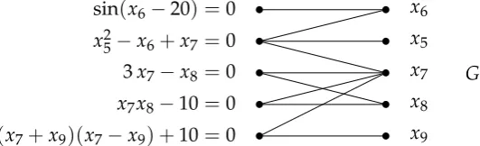
Definition 3.6. A well-constrained bipartite graphG = (V,E)with V =

L∪Iis calledirreducibleif every edge(`,i)∈Eis part of at least one perfect matching ofG.

sin(x6−20) =0

x2

5−x6+x7 =0

3x7−x8 =0

x7x8−10=0 (x7+x9)(x7−x9) +10=0

x6

x5

x7

x8

x9

[image:21.595.173.439.513.594.2]

G

Figure 3.3: A valid instance for the fine decomposition

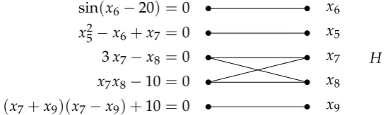
Definition 3.7. Thefine decompositionof a well-constrained bipartite graph G = (V,E) with V = L∪ I (see Section 2.2.1) consists ofq disjoint sub-graphsH1, . . . ,Hqconstructed as follows:

(22)

a perfect matching, i.e.

H= (V,{e∈E:eis in at least one perfect matching ofG}).

Now letH1, . . . ,Hqbe theqcomponents ofH. Obviously, every component

of H is irreducible. That is why H1, . . . ,Hq are also called the irreducible

components.

sin(x6−20) =0

x2

5−x6+x7 =0

3x7−x8 =0

x7x8−10=0 (x7+x9)(x7−x9) +10=0

x6

x5

x7

x8

x9

[image:22.595.169.442.251.333.2]

H

Figure 3.4: Example ofHconstructed from the instance of Figure 3.3

sin(x6−20) =0

x2

5−x6+x7 =0

3x7−x8 =0

x7x8−10 =0 (x7+x9)(x7−x9) +10 =0

x6

x5

x7

x8

x9

H1

H2

H3

H4

Figure 3.5: Example of a fine decomposition

An example ofHand the decomposition can be found in Figures 3.4 and 3.5 respectively. The fine decomposition has some useful properties that will be stated in a theorem.

Theorem 3.8. The fine decomposition satisfies the following conditions.

(a) The decomposition is unique.

(b) Every subgraph Hj∈ H1, . . . ,Hq is well-constrained.

(c) The subgraphs H1, . . . ,Hqcan be ordered (and renumbered) in such a way

that for every edge(`,i)with`_∈ H_j_∩L, i _∈H_k_∩I it holds that j_≥ k.

In words, (c) states that the subsystems corresponding toH1, . . . ,Hqcan be

[image:22.595.162.449.374.494.2]

(23)

only contains variables from

i:i∈ H1∪ · · · ∪Hj∩I . A consequence

is that this order is also an order of resolution of the associated subsystems of H1, . . . ,Hq. An ordering of our example system in Figure 3.5 could be

H3, H4, H1, H2.

To prove Theorem 3.8 more work is needed. See the next subsection.

Proof of Theorem 3.8

The proof is constructive and makes use of an arbitrary maximum match-ingMofG. It directly leads to an (polynomial) algorithm for the computa-tion of the fine decomposicomputa-tion.

Proof of (a) and (b). For (a) observe that the sets are well-defined thus the decomposition is unique for a specific bipartite graph.

(b) can be proven by contradiction. We know thatGhas a perfect matching M. By definition M is also a perfect matching of H. Suppose now that a subgraphHjis not well-constrained. ThenHjdoesn’t have a perfect

match-ing. Because Hjis a component ofHthat would mean thatHdoesn’t have

a perfect matching, which is a contradiction.

It would be useful to have a way to determine whether two vertices are in the same subgraph Hj. But first two auxiliary lemmas are needed. In these

lemmas,Mis a maximum (perfect) matching ofG. Lemma 3.9. The following statements are true.

(a) For every M-alternating tour T in G there exist(s) m ≥ 1 M-alternating cycle(s) C1, . . . ,Cmin G for which C1∪ · · · ∪Cmis connected and for which

it is true that every edge that appears in T also appears in C1∪ · · · ∪Cm.

(b) For an arbitrary set of m ≥ 1 M-alternating cycle(s) C1, . . . ,Cm in G for

which C1∪ · · · ∪Cm is connected there exists an M-alternating tour T in

G for which it is true that every edge that appears in C1∪ · · · ∪Cm also

appears in T.

(24)

M-alternating toursT1 where wherevis walked by 1 time andT2wherev

is walked byn−1 times by the following procedure.

LetT1 be the tour fromvfollowingTuntilvis reached again. Let the rest

of the tour beT2.

It is obvious that both T1 and T2 are M-alternating tours in G and every

vertex inTis inT1∪T2. T1andT2can be split up by the same procedure if

they contain vertices that are walked by a multiple number of times. Doing this over and over again results in the desired cyclesC1∪ · · · ∪Cm.

For (b), first sort and renumberC1∪ · · · ∪Cm such thatC1∪ · · · ∪Ciis

con-nected toCi+1fori=1, . . . ,m−1. LetT1=C1. Now proceed iteratively as

follows fori=1, . . . ,m−1.

LetTi be anM-alternating tour inGand letvi be a vertex withvi ∈ Tiand

vi ∈Ci+1. DefineTi+1as a tour starting invi, then start the tour by walking

all the way throughTi (starting with an edge in M) and then continue the

tour by walking all the way through Ci+1 (again starting with an edge in

M). It is obvious thatTi+1is an M-alternating tour inG.

NowTmis anM-alternating tour inGcontaining all vertices fromC1∪ · · · ∪

Cm.

Lemma 3.10. If there exists an M-alternating cycle C containing two vertices v1,v2∈ V then v1and v2are both an element of Hjfor a specific j.

Proof. LetM0_{be the symmetric difference}_M₄_{C. Now}_M0 _{is also a perfect}

matching. By definition all edges ofC = M4M0 _{are in}_H_{(each edge of}_C

is either in M or M0_{). Because} _C_{is a cycle it is obvious that} _v₁ _and_v₂ _are

connected and lie in the same component ofH.

Lemma 3.11. Two vertices v1,v2 ∈ V,v1 6= v2are both an element of Hj for a

specific j⇐⇒ v1 is matched to v2 by M or there exists an M-alternating tour T

containing both v1and v2(where T obviously has even length).

Proof. ⇐Ifv1is matched tov2byMthan obviouslyv1andv2are connected

inHand lie in the same component ofH.

So consider the case that there exists an M-alternating tour T containing bothv1andv2. By Lemma 3.9 we know that there existm≥1M-alternating

(25)

C1∪ · · · ∪Cm is connected. Lemma 3.10 implies that all vertices in an

M-alternating cycle are connected inH. That results in the fact that all vertices inC1∪ · · · ∪Cm, and thus inT, are connected inH.

⇒ It is known thatv1 andv2 are connected in H so there exists a path P

wherev1is the first vertex ofPandv2the last vertex. LetP0 = {e1, . . . ,em}

be P with all edges in M removed. Now, for i = 1, . . . ,m, let Mi be a

perfect matching containing ei. For all i = 1, . . . ,m take the symmetric

differenceSi = M4Mi. Because every vertex inSi can only have degree

0 or 2 the symmetric difference consists only of cycles. LetCi be the cycle

ofSi containingei. Notice thatCi isM-alternating and that the edges inM

adjacent to ei are also inCi. Because we know that either ei and ei+1 are

connected or there is an edge in Madjacent toei andei+1it follows thatCi

is connected toCi+1for alli=1, . . . ,m−1. By Lemma 3.9 it is known that

there exists anM-alternating tourTcontaining bothv1andv2.

Now it’s possible to prove condition (c) of Theorem 3.8.

Proof of (c). Suppose an ordering as stated in (c) would not be possible. The only way to achieve that is to have a “circular” sequenceH0

1, . . . ,Hm0 ,Hm0+1 =

H0

1 withm > 1 and H10, . . . ,Hm0 distinct such that there exists at least one

edge ij,`j+1withij ∈H0_j∩Iand`j+1 ∈ H0_j+1∩Lfor everyj∈ {1, . . . ,m}.

So suppose we have such a sequence. Consider an arbitrary edge ij,`j+1.

We know that ij,`j+1 is not matched by M or elseij and`j+1 would be

in the same Hj (by Lemma 3.11), which is a contradiction. Now look at

an edge ij+1,`j+2. By Lemma 3.11 it is known that there exists an

M-alternating tour Tbetweenij+1and`j+1. That implies there must exist an

M-alternating pathPj+1 betweenij+1and`j+1in H0j+1 where both the first

and last edge are inM. With this it is possible to construct anM-alternating tour(i1,`2)∪P2∪ · · · ∪(im,`m+1)∪Pm+1. But Lemma 3.11 then tells us that

all verticesij and`j+1forj = {1, . . . ,m}are in the same component of H,

which is a contradiction.

3.2.1 Implementation

(26)

Algorithm 3.2An algorithm for the fine decomposition

Input: A well-constrained bipartite graphG= (V,E)withV =L∪I Output:qsubgraphsH1, . . . ,HqwithV(H1)∪ · · · ∪V(Hq) =V 1 find a maximum matchingMofG

2 directed graphG0 _←(V,∅)

3 foreachedges(`,i)inGdo

4 add arc(`,i)toG0

5 foreachedges(`,i)inMdo

6 add arc(i,`)toG0

7 directed subgraphsG₁0, . . . ,G0_q_←strongly connected components ofG0 8 forjis1toqdo

9 Hj ←G

h

V(G0_j)i

This algorithm follows directly from Lemma 3.11. Every strongly con-nected component ofG0_{corresponds to either a single match (or edge) from}

Mor anM-alternating tour.

Lines 2 to 6 and lines 8 and 9 run inO(n+m)time wherenis the number of vertices and mis the number of edges inG. Line 7 also runs inO(n+

m) by using Tarjan’s Algorithm, see Tarjan (1972). The complexity of the

whole algorithm is determined by the complexity of finding a maximum matching in line 1. This can be done inO(m√n) time using the bipartite

matching algorithm of Hopcroft and Karp (1973).

Appendix B contains a recursive and a non-recursive version of Tarjan’s Algorithm. A nice property of using Tarjan’s Algorithm is that the order in which the strongly connected components are found is an order of resolu-tion for the subsystemsH1, . . . ,Hq.

Notice that lines 1 to 6 of Algorithm 3.1 and Algorithm 3.2 are the same. A consequence is that both algorithms can be merged very efficiently. How-ever, one must be aware of the fact that the input of the two algorithms differ. But when running Algorithm 3.2 withV1from Algorithm 3.1 as

(27)

3.3 The analysis component

Now that we have more information about the properties of the Dulmage-Mendelsohn, let us focus again on the interactive solver.

The interactive solver gives the current system of equations and its asso-ciated bipartite graph to the analysis component. This component uses the Dulmage-Mendelsohn decomposition to divide the system into the three subsystems V1, V2 and V3. V1 is well-constrained, V2 is over-constrained

andV3is under-constrained.

If the analysis component finds a non-empty V2, it stops and returns this

system to the solver. At least one of the equations inV2is either redundant

or contradicting and should be disabled by the solver. After that the system can be fed to the analysis component again.

After this check the analysis component is left withV1 andV3. It tries to

find irreducible components inV1 using the method described in

Subsec-tion 3.2.1. Then the solver determines which of the subsystems associated to the irreducible components can be solved without solving other subsys-tems first.

Finally the analysis component provides the solver with two lists: a list of solvable subsystems of V1 and a list of free parameters in V3 that can be

guessed without creating a non-emptyV2 in the resulting system of

equa-tions. By definition, all parameters inV3have this property. The solver can

either solve a subsystem using the partial solver of Section 4.2 or assign a (random) value to one of the free parameters. After this action the system can be analyzed by the analysis component again. Note that both actions will not introduce a non-emptyV2 component when the modified system

(28)

4

Newton methods

To solve a system of quations as described in Sections 2.4 and 3.3, the in-teractive solver has to solve (well-constrained) (sub)-systems of nonlinear equations. In this chapter we shortly describe the Newton method.

TheNewton methodis the most important algorithmic concept for solving a system of nonlinear equations

h(x) =0 (4.1)

whereh:Rn _→_Rn_,_h_∈_C1₍_Rn_,_Rn₎_{is a system of}_n_continuously

differen-tiable (nonlinear) functions ofnvariables.

The classicalNewton iterationfor computing a solution ¯xof (4.1) is

xk+1 =xk−Jh(xk)−1h(xk) (4.2)

whereJhis then×nJacobian matrix ofhandx0 ∈Rnis a (random) starting

vector. To findxk+1we simply have to solve the linear system

Jh(xk)(xk+1−xk) =−h(xk) (4.20)

forxk+1−xk and then calculatingxk+1fromxk.

It is well-known that the Newton iteration (4.2) is locally quadratically con-vergent to a solution ¯xofh(x¯) =0 if the regularity condition

Jh(x¯)is nonsingular (4.3)

is satisfied, i.e. under the assumption of (4.3) it holds that for any starting point x0 sufficiently close to ¯x, the iterates xk of (4.2) converge to ¯x with a

rate

(29)

wherecis a constant (see e.g. Faigle et al. (2002) for a proof).

The Newton method has one major drawback: the computation of the Ja-cobianJhis required. This is not possible in the SST framework because the

equations are implemented as “black box” functions. Besides that, every Newton iteration of (4.2) (or (4.20_{)) is at least of computational complexity}

O(n3).

It would be better to have a method with the following features: (a) only the values ofh(xk)are required.

(b) the computational complexity of each iteration is smaller thanO(n3₎_,

a better computational complexity would beO(n2).

(c) the iteratesxkare super-linear convergent, i.e.

kxk+1−x¯k

kxk−x¯k →0 ask →∞.

The so-called quasi-Newton method as described in the following section possesses these properties.

4.1 The quasi-Newton method

Thequasi-Newton methodis similar to the Newton method but it uses x_k+1= xk+α_kd_k

as update formula, wheredk =−B−k1h(xk),Bkis an approximation ofJh(xk)

andα_k is some step size.

To calculateBk+1one uses a low rank updateBk+1 =Bk+EkwhereEkis of

low rank (like rank(E)_≤2). The iteratesBk+1satisfy

Bk+1(xk+1−xk) =h(xk+1)−h(xk) (4.5)

which is called thequasi-Newton condition. This condition can also be writ-ten asBk+1sk =ykwhere

s_k = x_k+1−xk

(30)

To motivate the quasi-Newton condition (4.5) consider the Taylor expan-sion aroundxk+1:

h(xk)−h(xk+1) = Jh(xk+1)(xk−xk+1) +o(kxk−xk+1k).

So in (4.5) we obviously assume that Bk+1is an approximation of Jh(xk+1)

which satisfies the linear approximation

h(xk)−h(xk+1)≈ Jh(xk+1)(xk−xk+1).

The conceptual quasi-Newton method is described in Algorithm 4.1. Algorithm 4.1A conceptual algorithm for the quasi-Newton method Input: A functionh:Rn _→_Rn_,_h_∈_C1₍_Rn_,_Rn₎_{, a point}_x

0∈Rnand a

number of iterationsm Output: A vectorxm ∈Rn 1 B₀_←an approximation ofJ_h 2 forkis0tom₋1do

// update x_k+1

3 d_k _{← −}B−_k1h(xk) 4 x_k+1←xk+dk

// update approximation of Jacobian

5 B_k+1 ←Bk+Ek // or B_k−₊1₁ ←B−_k1+E˜_k

To possibly enlarge the region of attraction instead of line 4 of Algorithm 4.1 we can perform a step with line-minimization

α_k ← a solution of minα∈Rkh(xk+αdk)k

2

xk+1 ←xk+α_kd_k (4.6)

An update formula of particular interest is due to Broyden (1965). His fa-mous update formula

Bk+1= Bk+ (yk−Bksk)s T k

sT ksk

| {z }

Ek

(31)

or equivalently

B−1

k+1 =B−k1+

s_k₋B−1

k yk

sT

kB−k1

sT kB−k1sk

| {z }

˜

Ek

(4.70₎

is known as Broyden’s “good” update formula. As the name suggests he also proposed an update formula known as Broyden’s “bad” update for-mula:

B_k+1 =Bk+ (yk−Bksk)y T kBk

yT

kBksk (4.8)

or equivalently

B−1

k+1= B−k1+

sk−B_k−1yk

yT

k

yT

kyk . (4.8

0₎

Broyden (2000) gives the following explanation for the names of the formu-las: the formula is referred to as “good” due to its better numerical perfor-mance relative to another formula that I also presented in (1965), which has become to be known as the “bad Broyden” update. Dennis and Schnabel (1980) discuss these two updates and their relations to the DFP and BFGS updates.

4.1.1 Convergence results

The quasi-Newton method with Broyden’s update (4.7), also called Broy-den’s method, leads to a superlinearly convergent method.

Theorem 4.1(Convergence result). Let h be a C1_{-function in a (open)}

neighbor-hood ofx such that h¯ (x¯) =0and Jh(x¯)is nonsingular. Then for Broyden’s method

and the method from Algorithm 4.1 without using(4.6)the following holds. There exist constantsδ,e>0such that for any x0,B0satisfying

kx0−x¯k<δand kB0−Jh(x0)k<e

the iterates xkconverge tox superlinearly.¯

(32)

-10 -8 -6 -4 -2 0 2 4 6 8 10 -20

-15 -10 -5 0 5 10 15 20

converges to negative solution converges to positive solution y= 3₂x+1

[image:32.595.138.471.107.398.2]

1= 1₄x2₋₁₆1y2

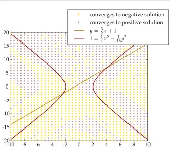
Figure 4.1: Behaviour of convergence of Broyden’s method on System 4.10

Note that in the case wheren=1, the quasi-Newton condition

Bksk−1 =yk−1orB−_k1= _ysk−1

k−1 =

xk−xk−1

h(xk)−h(xk−1)

yields the so calledsecant method

xk+1 =xk− _h₍_xxk−xk−1

k)−h(xk−1)h(xk). (4.9)

It is also proved by Gay (1979) that when Broyden’s method is applied to a linear system, it terminates in 2nsteps. This is a usefull property for the solver. When a linear system has to be solved, there is no need to use a specialized method for linear systems.

(33)

of equations

  

 

−3₂x1+x2 =1

1 4x12−

1

16 x22 =1   

 

(4.10)

which has(−2.375,−2.563)and(4.090, 7.134)as solutions. One could

cre-ate a grid of starting points and determine for every starting point to which solution it converges. This has been done in Figure 4.1. There is no clear global convergence behaviour, except (according to Theorem 4.1) in a small neighbourhood of the solutions. An interesting sidenote is that Broyden’s method converged for all starting points in Figure 4.1 in less then 29 itera-tions.

4.2 The partial solver

The partial solveris the component of the SST framework that used Broy-den’s method to solve the (irreducible) subsystems that are returned from the analysis compontent of Section 3.3. By definition these subsystems are well-constrained and thus consistent. That also means that with a “high probability” h is regular, i.e. all solutions ¯x of h(x¯) = 0 satisfy the regu-larity condition (4.3). So by Theorem 4.1, if solutions ¯x of h(x¯) = 0 exist,

with high probability Broyden’s method will converge to them when the starting point is close enough to the solution.

If a solution does not exist or the random starting point is too far from a so-lution, Broyden’s method might not converge. If the iterates have not con-verged after a specified number of iterations, the partial solver will restart with another random starting point. After a specified number of restarts the partial solver will report to the solver that it was not able to solve the subsystem.

In this situation, probably the best choice for the interactive solver is to discard the current assignment of parameters, enable all rules again and start all over. Because the choices for assigned parameters and disabled rules have consequences for the type of encountered subsystems, it could be well possible that the interactive solver will be able to solve all encoun-tered subsystems in the next attempt.

(34)

(35)

5

Bandwidth reduction

A major problem of manipulating large sparse matrices is that a lot of stor-age space and computing time are needed. One way of dealing with this is by permuting the rows and columns of the matrix such that it becomes a band matrix. A band matrix is a sparse matrix whose nonzero elements are within a certain distance from the main diagonal. When such permu-tations result in a band matrix of small bandwidth, considerable savings in both storage space and computing time are possible using banded algo-rithms, see for example Martin and Wilkinson (1967). A natural question that arises is what the smallest possible bandwidth for a given matrix is. A lot of research has been put into reducing the bandwidth of symmetric matrices. However, unsymmetric matrices didn’t get much attention. In the SST project unsymmetric matrices are more common, so this problem is worth investigating.

In Subsections 5.1 and 5.2, the symmetric and unsymmetric bandwidth minimization problem will be introduced respectively. Subsection 5.3 will give a short overview of the available literature of both problems. In Sub-section 5.4 a proof will be presented showing that the unsymmetric band-width minimization problem is NP-complete. A popular class of algo-rithms concerning bandwidth reduction, the level set algoalgo-rithms, will be treated in Subsection 5.5 and some more traditional heuristics are covered in Subsection 5.6. A short overview of the software written for this thesis can be found in Subsection 5.8 and finally, the computational results can be found in Subsection 5.7.

5.1 Symmetric case

(36)

1 2 3 4 5 6 7 8 9 10

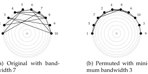
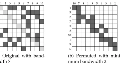
(a) Original with band-width 7 1 5 7 2 4 8 6 10 3 9

1 5 7 2 4 8 6 10 3 9

[image:36.595.187.427.295.415.2]

(b) Permuted with mini-mum bandwidth 3

Figure 5.1: Symmetric matrix

10 9 8 7 6 5 4 3 2 1

Figure 5.2: Graph representation of Figure 5.1

Given a symmetric matrix A =

aij ∈ Rn×n, thesemi-bandwidthof matrix

Ais defined asbs = max |i−j|:aij 6=0. In the literature different

defi-nitions for the bandwidth of a matrix are used. Usually the bandwidth is eitherbs, 2bs or 2bs+1. In this thesis thebandwidthof a symmetric matrix

is simply defined asb=bs, the semi-bandwidth.

The(symmetric) bandwidth minimization problem(BMP) is defined as follows: given a symmetric matrix A a permutation of the rows and columns of A (where both permutations are the same to preserve symmetry) must be found such that the bandwidth, b, is minimized. In other words, all nonzero elements ofAshould be in a band that is as close as possible to the main diagonal.

In the context of graphs, given a graphG = (V,E), whereV is the vertex set with|V| = nandEis the edge set, the bandwidth minimization

(37)

the length of the longest edge when the vertices are ordered on a line with unit distance between consecutive vertices.

The matrix bandwidth minimization problem and the graph bandwidth minimization problem are interchangeable using A as the (vertex-vertex) adjacency matrix ofG.

Figure 5.1 shows an instance of the symmetric bandwidth minimization problem. The nonzero elements of the matrix are shown as dark grey squares and the elements on the main diagonal are shown as light grey squares. Figure 5.2 shows the graph representation of the same problem. The points of the graph are ordered on half a circle instead of on a line to give a better visualization of the length of an edge.

5.2 Unsymmetric case

The main focus of this thesis will be a generalisation of the bandwidth minimization problem, namely the unsymmetric bandwidth minimization problem. In this problem, matrix Ais allowed to be unsymmetric. While such a matrix is allowed to be non-square, the focus will be on square un-symmetric matrices.

Because of the loss of symmetry another definition for the bandwidth is needed. Given a matrix A = [a`i] ∈ Rm×nwhere` ∈ {1, . . . , m}andi ∈

{1, . . . , n}let us define thelower bandwidth b`as max{`−i:a`i 6=0, ` >i}

and theupper bandwidth buas max{i−`: a`i 6=0, ` <i}. Different

defini-tions for the bandwidth are possible. Common choices are max(b`,bu),

b`+bu,b`+bu+1 andb`+bu+min(b`,bu). In this thesis thebandwidth b

of an unsymmetric matrix is simply defined as max(b`,bu). Let us denote

by b(A) the bandwidth of matrix A. Note that for symmetric matrices,

b=max(b`,bu) =bs.

Theminimal bandwidthofAis defined by

β(A) = min

πL∈Sm,πI∈Snb

(haπL(`)πI(i)

i

)

where Sn and Sm are the symmetric groups of permutations of

respec-tively nand mobjects. Soβ(A)denotes the smallest bandwidth that can

(38)

1 2 3 4 5 6 7 8 9 10

10 7 8 1 9 5 6 3 4 2

[image:38.595.158.443.114.427.2]

Figure 5.3: Unsymmetric matrix

10, 10 9, 9 8, 8 7, 7 6, 6 5, 5 4, 4 3, 3 2, 2 1, 1

(a) Original with bandwidth 7

6, 2 9, 4 1, 3 10, 6 8, 5 3, 9 7, 1 2, 8 5, 7 4, 10

(b) Permuted with minimum bandwidth 2

Figure 5.4: Graph representation of Figure 5.3

The unsymmetric bandwidth minimization problem (UBMP) is to determine

β(A), given the matrixA.

In the context of graphs, consider a bipartite graph G = (V,E), where V = L∪ I is the vertex set and E ⊆ L×I is the edge set. L and I are the vertex classes of the bipartite graph with _|L_| = m and_|I_| = n. The

bipartite graph bandwidth minimization problemis to find a bijective labeling pL(v): L→ {1, . . . , m}and a bijective labelingpI(v): I → {1, . . . , n}that

minimizes max{|pL(`)−pI(i)|:(`,i)∈E}, or, equivalently, minimize the

length of the longest edge when the vertices are ordered with unit distance on two parallel lines, one for each vertex class, where the lengthl(e)of an

edgeeis the Euclidean distance between its two incident vertices projected on either of the two lines.

The unsymmetric bandwidth minimization problem and the bipartite graph bandwidth minimization problem are interchangeable: each row` of

[image:38.595.193.425.131.256.2]

(39)

corre-sponds to a vertexi∈ I;a`i is nonzero iff(`,i)∈ E.

Figure 5.3 shows an example of the unsymmetric bandwidth minimization problem. Figure 5.4 shows the graph representation of the same problem. Again, the vertices of the graph are ordered on a half circle instead of on a line to give a better visualization of the length of an edge. Furthermore, the vertex corresponding to row positionjis placed at the same coordinates as the vertex corresponding to column positionj. For example 3, 9 means that both the vertices corresponding to row 3 and column 9 are located at that coordinate.

Note that the graph representation as used in Figure 5.4 is only usable with the bandwidth defined as max(b`,bu). When another bandwidth definition

is used, one has to differentiate between edges where the column vertex is located to the left of the row vertex and edges where the column vertex is located to the right of the row vertex.

5.3 Literature

Most available literature covers the symmetric bandwidth minimization problem, which will be referred to as the BMP from now on. Since 1976 this problem is known to be NP-complete, due to Papadimitriou (1976). Unger (1998) even showed that, for any constant k, it is NP-complete to find ak-approximation of the BMP, i.e. finding a (polynomial) approxima-tion algorithm that guarantees that the approximaapproxima-tion will have a band-width smaller than kβ (k times the smallest possible bandwidth) would

yield P=NP.

Nevertheless Corso and Manzini (1999) developed two algorithms to find an exact solution for the BMP. Because the running time of these algorithms can be very large for large problem instances, many efforts have been done to develop heuristic algorithms. These algorithms can be much faster, but don’t guarantee optimal solutions. That is why they are usually referred to asbandwidth reduction algorithms.

(40)

level sets in this algorithm led to the development of theGPS algorithm(by Lewis (1982)), the Sloan algorithm(by Sloan (1989)), the JCL algorithm (by Luo (1992)) and the more recentWBRA algorithm(by Esposito et al. (1998a)). More recently, another class of algorithms for the BMP has been investi-gated: the class of metaheuristics. The first metaheuristic applied to the BMP wassimulated annealing, due to Dueck and Jeffs (1995). A recent im-provement of this approach has been proposed by Rodriguez-Tello et al. (2008). Esposito et al. (1998b) and Martí et al. (2001) usedtabu searchto re-duce the bandwidth of a symmetric matrix. Piñana et al. (2004) presented the results of applying a greedy randomized adaptive search pocedure combined with a path relinking strategy (GRASP-PR). And finally, Pop and Matei (2011) developed a heuristic based ongenetic programming.

As far as we know, little research has been done for the unsymmetric band-width minimization problem, which will be referred to as the UBMP from now on. Esposito et al. (1998b) describe an adjustment to Tabu Search and the WBRA algorithm (a heuristic for the BMP) to incorporate unsymmetric matrices. Reid and Scott (2006) developed methods to reduce a quantity called thetotal bandwidth, which is defined as min(b`,bu) +b`+bu.

5.4 NP-completeness of the UBMP

The BMP is proved to be NP-complete, due to Papadimitriou (1976), by reducing 3-SAT to a generalized problem where a number of k edges are restricted by a bandwidth of 2b−1 instead ofb. Another reduction is ap-pliedktimes such that in the resulting problem all edges are restricted by a bandwidth ofb0_{. In this section, the NP-completeness of the UBMP will be}

investigated and also proved by reducing 3-SAT to it. Some key concepts from the original proof will be used. However, a direct reduction from 3-SAT will be presented without using an intermediate problem.

(41)

1 2 3 4 5 6

(a) Original with band-width 4 1 2 5 3 4 6

1 2 5 3 4 6

(b) Symmetrically per-muted with minimum bandwidth 2 2 4 1 3 5 6

6 5 3 1 4 2

(c) Unsymmetrically per-muted with minimum bandwidth 1

Figure 5.5: Symmetric matrix

For the UBMP to be NP-complete, it has to be in NP. Recall that for a matrix A= [a`i],β(A) =minπL∈Sm,πI∈Snmax(|πL(`)−πI(i)|:a`i 6=0).

Definition 5.1. Theunsymmetric bandwidth minimization decision problem (UB-MDP) is the following: given a matrix A∈ Rm×n_{and an integer}_b

d > 0, is β(A)≤b_d?

Lemma 5.2. The UBMDP is in NP.

Proof. Let the permutation of rowsπLand the permutation of columnsπI

be the certificate of a “yes” instance. Now the “yes” instance can be verified by checking_|πL(`)−πI(i)| ≤ bdfor all{`,i|a`i 6= 0}. This can be done in

O(mn)time.

Corollary 5.3. The UBMP is an NP-optimization problem.

Proof. By Lemma 5.2 the decision problem of the UBMP is in NP.

To show that the UBMP is NP-complete, its NP-hardness must be proved as well. For this proof, a definition of 3-SAT is necessary. The (exactly) 3-satisfiability problem(3-SAT) is defined as follows: givenndifferent Boolean variables x1, . . . , xnandr clausesF1, . . . , Fr each containing exactly 3

dif-ferent literals f1, f2, f3 ∈ {x1, . . . , xn, ¯x1, . . . , ¯xn}, does an assignment of

TRUEandFALSEto the variablesx1, . . . , xnexist such that all clauses

eval-uate toTRUE?

An instance of 3-SAT withn=5 andr =3 could be for example (x1∨x¯2∨x¯3)∧(x¯1∨x3∨x¯4)∧(x2∨x4∨x¯5).

(42)

M0

P0 _Q0

H0

m1 mh

vn

v2

v1 v¯1 v¯2 v¯n

m0

1 m0h

v0_n

v0 2

v0

1 v¯10 v¯20 v¯n0

[image:42.595.141.477.125.265.2]

· · · · · · · · · · · · M P Q P Q H · · · · · ·

⇒

Figure 5.6: Bipartite graph(H,H0)

Theorem 5.4. The UBMP is NP-hard.

Proof. By reducing 3-SAT to the decision problem UBMDP. Consider an in-stanceSof 3-SAT withnBoolean variablesx1, . . . , xnandrclausesF1, . . . , Fr.

An instanceUof the UBMDP withbd =n+4 will be created such thatSis

solvable iffUis a “yes” instance.

For a better understanding of the proof, the bipartite graph representation of the problem will be used. The most important building block ofUwill be the bipartite graph(H,H0₎_{, as shown in Figure 5.6.} ₍_H,_H0₎_{can be}

con-structed as follows: for each variable xi in S,i = 1, . . . , n, add 2 vertices

v_i, ¯v_i to Handv0

i, ¯vi0 to H0. Also add the vertex sets M = {m1, . . . , mh}to

HandM0 ₌ m0

1, . . . , m0h toH0 withh=2 orh=3. Now connect eachvi

and ¯vito allm0 ∈ M0. The verticesvi, ¯vi will be referred to asliterals.

The rest of the construction ofUas given below will force (H,H0₎_{to have}

certain properties in a valid solution ofU:

(a) The verticesM= _{m1, . . . , mh}will be next to each other in the

mid-dle of H and the vertices M0 ₌ m0

1, . . . , m0h will be next to each

other in the middle ofH0_. _M_{will be positioned exactly above} _M0_.

(b) Exactly n literals from {v1, . . . , vn, ¯v1, . . . , ¯vn} are to the left of M,

call this subsetP, and exactlynliterals are to the right ofM, call this subsetQ.

(c) Not bothviand ¯viare inP, i.e.viand ¯viare at different sides ofM.

(43)

k2

k1 k3 kn+3 kn+4 kn+5

· · ·

k0 2

k0

1 k03 k0n+3 kn0+4 kn0+5

· · ·

K0

K

⇒

Figure 5.7: Bipartite graph(K,K0)

a3

a1 a4

a0 3

a0

1 a04

a2

a0

2 A0

A

[image:43.595.160.460.109.392.2]

⇒

Figure 5.8: Bipartite graph(A,A0₎

Clearly the last property will be enough to prove the theorem. To enforce these properties, two more building blocks are needed. One of them is the bipartite graph(K,K0)(see Figure 5.7). This is a complete bipartite graph

withK= _{k1, . . . , kn+5}andK0 =k01, . . . , k0n+5 . Because there is an edge

between all vertices ofKand all vertices ofK0_,_K_{will be exactly positioned}

aboveK0_{in a valid solution of}_{U. Note that a bipartite graph consisting of}

one component can only be at one side of(K,K0).

The last building block is the bipartite graph(A,A0)(Figure 5.8). It consists

of just A = _{a1, . . . , a4}andA0 = {a01, . . . , a04}. The total construction of

U will force Ato be exactly positioned above A0 _{in a valid solution of}_U.

Also the vertices ofAandA0_{will be positioned next to each other in a valid}

solution.

Now the bipartite graph U can be constructed. Take n copies of (H,H0₎

withh = 3 toUand call them(H1,H10), . . . , (Hn,Hn0)and addr copies of

(H,H0)with h = 2 and call them Hn+1,H_n0+1

, . . . , (Hn+r,Hn0+r). Then

(44)

P0

2 Q02

H0

1 A01

P0 3

H0

2 A02

· · ·

A0

n+r

P0 1

Q0 1

H0

n+r

P1 Q1

H1 A1

P2 Q2

H2 A2

· · ·

An+r

Pn+r Qn+r

Hn+r

K0 1

K1

Q0

n+r

K0 2

K2

Figure 5.9: Prearrangement ofU

M0

j Pj0+1 Q0j+1 M0j+1

Mj

Pj Qj Pj+1 Mj+1 Qj+1

[image:44.595.106.504.115.390.2]

· · · · A0 j Aj · · · · · · · · · · · · · · · ·

Figure 5.10: Edges added toU, wherej=1, . . . , n+r−1

order

K1,K10, H1,H10, A1,A01, . . . , Hn+r,Hn0+r, An+r,A0n+r, K2,K02.

Let us rearrange each bipartite graph(Hi,H_i0)such that(Mi,M_i0)is exactly

in the middle of(Hi,Hi0). And within each vertex setH0ireplace each vertex

set P0

i withQ0i,Q0j with Pj0+1 andQ0n+r withP10, wherei = 1, . . . , n+rand

j=1, . . . , n+r₋1, see Figure 5.9.

As Figure 5.9 suggests, as many edges as possible will be added betweenK1

andM0

1,K01andM1,MiandAi0,M0iandAi,AjandM0j+1,A0jandMj+1,An+r

and K0

2, A0n+r and K2, M1 and Q0₁, and Mn+r and P₁0 under the condition

that an added edge e will have a length l(e) _≤ n+4 given the current arrangement.

For each literal v ∈ Pj∪Qj, connect with it its corresponding literal v0 ∈

P0

j+1∪Q0j+1and connectv0 with its corresponding literalv00 ∈ Pj+1∪Qj+1,

as shown in Figure 5.10, wherej=1, . . . , n+r₋1.

(45)

not in(K1,K₁0)or(K2,K₂0)is part of a connected component adjacent to both (K1,K10)and(K2,K20). Hence, in a valid solution ofU,(K1,K01)and(K2,K20)

must be arranged at the outer ends. Without loss of generality, we can say that (K1,K10)will be placed all the way to the left and(K2,K02)all the way

to the right.

Because of the edges that were added in our construction, see Figure 5.9, and the fact that(K1,K10)and(K2,K20)will be arranged at the outer ends,

the subgraphs

M1,M10, A1,A01, M2,M02, . . . , An+r−1,A0n+r−1, Mn+r,M0n+r

will stretch out leaving exactly npoints of “free space” around them (this free space will be occupied by the vertices of Pi, Qi, P_i0 and Q0_i). This

means that each subgraph (Hi,Hi0) in U already has Property (a), with

i = 1, . . . , n+r. The edges that were added in Figure 5.6 restrict each

subgraph(Hi,H_i0)inUto have Property (b) and the property that vertices

that were added inPi∪Qiwill stay inPi∪Qiin a valid solution ofU.

Furthermore, the edges added in Figure 5.10 force each partition of literals fromPi∪Qi overPiandQi to be the same for all subgraphs(Hi,Hi0). Note

that the precise arrangement of literals within Pi and Qi doesn’t have to

be the same for all subgraphs (Hi,Hi0). For i = 1, . . . , n−1, due to the

choiceh=3, a literal fromHican move at most 1 position forward inHi+1.

And for i = n, . . . , n+r−1, where h = 2, a literal from Hi can move

at most 2 positions forward in Hi+1. This freedom will be necessary to

enforce the last two properties. However, our construction will assure that the arrangement of literals withinP0

j+1will be the same as withinPj+1and