Peninsula, Somerset: Development and
application of a multi-proxy sea-level transfer
function for the Severn Estuary region
A thesis submitted in partial fulfilment of the requirements of the University of the West of England, Bristol for the degree of Doctor of Philosophy
Elizabeth Grace Elliott
Acknowledgements
There are a great many people who have been an incredible help to me in completing my
doctoral thesis, whether by offering practical assistance or simply encouragement. I was
lucky to share an office with some wonderful characters, and while I couldn’t list everyone
who passed through the FET postgraduate research offices over the past four years, I must
give particular thanks to Billy, Geoff, Caroline, Cuong, Amy, Sarah, Simon, Kate and Ben for
their friendship and encouragement during the time we spent as research students together.
Thanks also to lab technicians Emma Brown and Andy Geary, not only for their help and
advice in the laboratory, but also for joining me in the field, along with Chris Spencer, Chris
Parker and Anne Bridle.
I’m grateful to Richard Mourne for all of the advice and ideas he gave me during the
progression process of the PhD, and to Wendy Woodland and David Case for the significant
contributions they made as supervisors.
I reserve my greatest of thanks for Chris Spencer who, as my director of studies, has
been unendingly supportive and encouraging, and who was quite happy to wade out into the
Severn Estuary to help me collect sediment samples.
I acknowledge the Department of Geography and Environmental Management, University
of the West of England, Bristol, for funding this research degree and would like to thank my
internal and external examiners Nevil Quinn and Jason Kirby for their advice.
Finally, many thanks to my parents for putting up with my eccentric career choices, and
at home, to Tom, for lending me the benefit of his experience as a PhD student, for giving
me so much support and for putting up with the many weekends that were taken up by the
thesis in the last few months!
This thesis presents a multi-proxy reconstruction of Holocene sea-level change at the Steart
Peninsula in Bridgwater Bay, Somerset. Single- and multi-proxy transfer functions were
developed from diatom and foraminifera training data from two sites on the Severn Estuary
coast. Constrained and partial constrained ordination estimated that 5.5% of the intertidal
diatom variation and 11.4% of the intertidal foraminifera variation in the training sets was
explained independently by elevation within the tidal frame.
Foraminifera provided more favourable transfer function prediction statistics but were low
in abundance in parts of the intertidal zone, resulting in a smaller than optimal training set.
The preferred transfer function combined diatom and foraminifera data to optimise prediction
statistics and intertidal coverage.
An 11.22m fossil core was retrieved from the Steart Peninsula for stratigraphic and
mi-cropalaeontological analyses. Analogue matching revealed that combining the two proxies
increased the number of fossil samples with good or fair modern analogues in relation to
the single proxies separately. The preferred multi-proxy transfer function was applied to the
fossil micropalaeontological data.
The sediment stratigraphy, biostratigraphy and transfer function-based estimates
indi-cated an overall rise in relative sea-level of about 13m between 7,582-7,345 and 1,804-1,690
cal. years before present (cal. yr BP), beginning with an initial rapid phase of sea-level
rise and silty clay deposition in a minerogenic saltmarsh environment. Between 6,188-6,007
and 3,942-3,759 cal. years BP three main fluctuations in marine influence occurred, allowing
organic upper saltmarsh conditions to develop periodically, but the data scatter and large
vertical error bars prevent a detailed interpretation of absolute sea-level change. Diatoms
and foraminifera were sparse or absent between 4,053-3,869 and 1,927-1,806 cal. years BP.
Finally, foraminifera assemblages indicated a possible tidal flat environment and increase in
marine influence between 1,927-1,806 and 1,682-1,619 cal. years BP.
This research concludes that multi-proxy methods have the potential to improve the
iii
curacy and precision of relative sea-level reconstruction in an extremely macrotidal setting
such as that of the Severn Estuary, but that a number of issues such as sediment
autocom-paction and possible Holocene tidal range changes need to be quantified in order for the broad
1 Introduction 1
1.1 The significance of Holocene sea-level research . . . 1
1.2 Sea-level change at the Steart Peninsula and the wider Somerset Levels . . . 5
1.3 Thesis aims and objectives . . . 7
2 Sea-Level Variability and Reconstruction 9 2.1 Quaternary climate and sea-level variability . . . 9
2.2 Holocene climate and sea-level variability . . . 12
2.3 Sea-level indicators . . . 15
2.4 Sea-level reconstruction . . . 23
2.5 Quantitative environmental reconstruction . . . 26
2.6 Implementation of the transfer function approach in sea-level studies . . . 32
2.7 Vertical and horizontal sources of error . . . 49
2.8 Chapter Summary . . . 55
3 The Holocene Environmental History of the Somerset Levels 57 3.1 The Somerset Levels . . . 57
3.2 Holocene evolution of the moors . . . 59
3.3 Holocene stratigraphy of the Somerset Levels . . . 61
3.4 Human occupation and the draining of the Somerset Levels and Moors . . . . 64
3.5 Holocene sea-level change in the Somerset Levels and Severn Estuary . . . 66
3.6 Bridgwater Bay . . . 77
3.7 The Steart Peninsula . . . 77
3.8 Chapter summary . . . 86
4 Methodology 88 4.1 Contemporary intertidal microorganisms and environmental factors . . . 88
4.2 Quantifying the role of environmental factors in explaining intertidal micro-faunal variation . . . 104
4.3 Developing a multi-proxy sea-level transfer function . . . 112
4.4 Reconstructing Holocene sea-level change in at the Steart Peninsula . . . 116
4.5 Key assumptions . . . 123
4.6 Limitations of the transfer function approach . . . 125
5 Sea-level transfer function development 130 5.1 Contemporary intertidal microorganisms and environmental measures . . . . 130
5.2 Quantifying the role of elevation in explaining intertidal microfaunal variation 143 5.3 Transfer function development: single and multi-proxy . . . 150
5.4 Chapter summary . . . 160
6 Sea-level transfer function analysis and discussion 162 6.1 Diatom and foraminifera training sets . . . 162
Contents v
6.2 Combining proxies . . . 170
6.3 Species-environment relationships . . . 172
6.4 Transfer function development . . . 176
6.5 Chapter summary . . . 180
7 Palaeoenvironmental evidence from the Steart Peninsula 181 7.1 Sediment stratigraphy and fossil microfauna . . . 181
7.2 Core chronology . . . 196
7.3 Modern analogues . . . 198
7.4 Selecting the most appropriate transfer function . . . 204
7.5 Chapter summary . . . 215
8 Holocene environment and sea-level reconstruction at the Steart Peninsula216 8.1 Application of the prefered transfer function . . . 216
8.2 Stratigraphic interpretation . . . 222
8.3 Foraminifera-based interpretation . . . 223
8.4 Diatom-based interpretation . . . 224
8.5 Transfer function-based interpretation . . . 225
8.6 Integrated interpretation . . . 227
8.7 Evaluating the quantitative sea-level reconstruction . . . 230
8.8 Sea-level change in Bridgwater Bay . . . 233
8.9 The wider Severn Estuary region . . . 238
8.10 Limitations . . . 243
8.11 Future research possibilities . . . 245
9 Conclusions and implications 251
1.1 Map of the Severn Estuary levels, showing places mentioned in the text. . . 6 1.2 Holocene sea-level rise in the Bristol Channel, from Kidson and Heyworth (1976). 7
2.1 Stacked Quaternary δ18O record for the last 3.6 million years, from Lisiecki and Raymo (2005). . . 11 2.2 Correspondence between (a)δ18O record from east equatorial core V19-30, from
measurements of benthic Uvigerina senticosa and (b) eustatic sea-level curve for the Huon Peninsula, New Guinea, over the last 250,000 years. Adapted from Chappell and Shackleton (1986) by Masselink and Hughes (2003). Reproduced with permission from Taylor & Francis. . . 12 2.3 Eustatic sea-level curve for the Holocene. . . 14 2.4 Floral and microfaunal zones of sites in Southern California and Chezzetcook Inlet,
Nova Scotia, from Scott and Medioli (1978). . . 20 2.5 Fossil diatom zonation based on salinity preferences from Frosta, Nord-Trøndelag,
Norway. Adapted from Kjemperud (1981) by Palmer and Abbott (1986). . . 22 2.6 Relative mean sea-level curve for North Wales, from Robertset al. (2011). . . 25 2.7 Venn diagrams illustrating the concept of different analogue situations, from
Dela-court and DelaDela-court (1991). . . 29 2.8 The principle parts of quantitative palaeoenvironmental reconstruction, from Birks
et al. (2010). . . 30 2.9 Relative changes in mean tidal level (MTL) at Machiasport during the past 6,000
years, from Gehrels (1999). . . 35 2.10 Relative sea-level changes at Vidarh´almi, Iceland, from Gehrels et al.(2006b). . . 36 2.11 Number of live, dead and total foraminifera specimens for all species from Cowpen
Marsh, between 1 May 1995 and 3 May 1996, from Horton and Edwards (2006). 38 2.12 Pie charts showing the total variation of the Horton and Edwards (2000) (a)
foraminifera and (b) diatom training sets in explained and unexplained portions, and components representing the unique contributions of standardised water level index (SWLI), salinity, loss on ignition, vegetation cover, pH, grain size and inter-correlations among gradients. . . 46 2.13 Age-altitude graph of sea-level index point (SLIP) at Holkham, North Norfolk
using the Horton and Edwards (2000) foraminifera-based transfer function. . . . 47 2.14 Plots of (a) all validated SLIPs and (b) SLIPs from basal peats, from 52 sites
in Great Britain, for the past 10,000 years, compared with the ranges of relative sea-level changes from the models of Lambeck (1995) and Peltieret al. (2002) . . 52 2.15 SLIPs for sites in southern England and Wales plotted as calibrated ages against
changes in sea-level relative to present Ordnance Datum (OD) (m), from Shennan and Horton (2002). . . 53
3.1 The Severn Estuary Levels, rivers and key settlements. Adapted from Allen and Haslett (2002) with permission from SAGE Publications. . . 58
List of Figures vii
3.2 The extent of ice cover in the British Isles during the Devensian glacial. Repro-duced from Bowenet al. (2002) with permission from Elsevier. . . 60 3.3 Cross section showing the typical morphology of the four marsh units in the Severn
Estuary. Adapted from Allen (2004) with permission from SAGE Publicatinos. . 64 3.4 Height/age Holocene sea-level curve for South West England. From Hawkins
(1971a). . . 67 3.5 Holocene sea-level rise in the Bristol Channel, from Kidson and Heyworth (1976). 69 3.6 70 SLIPs for the Bristol Channel region plotted as calibrated age against change
in sea-level relative to present (m), from Shennan and Horton (2002). . . 71 3.7 Late Holocene relative land-/sea-level changes in Great Britain (mm/yr), from
Shennan and Horton (2002). . . 72 3.8 Stratigraphy of the Rookery Farm transect at Nyland Hill, Somerset, from Haslett
et al. (1998). . . 73 3.9 Map of Bridgwater Bay and the locations mentioned in the text. . . 79 3.10 Historic OS maps illustrating the changes at Stert Point that occurred between
the 1890s and 1900s. . . 80 3.11 Locations of boreholes in Bridgwater Bay and the Somerset Levels, from Kidson
and Heyworth (1976). . . 82 3.12 Section through the beach at Stolford, from Kidson and Heyworth (1976). . . 83 3.13 Inland extension of the sequence shown in Figure 3.12, from Kidson and Heyworth
(1976). . . 84 3.14 Section across the mouth of the River Parrett, from Kidson and Heyworth (1976). 85 3.15 Sea-level index points (SLIPs) from five publications on Holocene sea-level in the
Severn Estuary region. . . 87
4.1 Maps of (a) the Severn Estuary/Bristol Channel region and the sites of the two modern transects, (b) the site of transect ST1 at Stert Flats and (c) the site of transect BT1 at Beachley Point. . . 93 4.2 Annotated photographs of Stert Flats. . . 95 4.3 Annotated photographs of Beachley Point. . . 96 4.4 A: a linear response model; B: a unimodal response model. From Daleet al.(2002).107 4.5 The two main types of distortion caused by correspondence analysis (CA) ordination.108 4.6 Illustration of canonical correspondence analysis (CCA) (a) sample-environment
and (b) species environment biplots of foraminifera and environmental data from Cowpen Marsh on the Tees Estuary. From Horton and Edwards (2006). . . 110 4.7 Location of the coring site near Wall Common on the Steart Peninsula. . . 117 4.8 Classification scheme for cognition and ignorance, knowledge and uncertainty.
Adapted from Jackson (2012) with permission from Elsevier. . . 126 4.9 Estimates of the strength of analogy for samples from a core from Salvo, North
Carolina, with modern training set assemblages. Reproduced from Kemp et al. (2009a) with permission from Elsevier. . . 128
5.1 Variation in loss on ignition (LOI), conductivity and pH across transects BT1 and ST1, and the main floral species present, plotted against SWLI. . . 132 5.2 Variation in the percentage abundance of diatom species across transect ST1. . . 133 5.3 Variation in the number of living and dead foraminifera counted per 2cm3 of
sediment across transect ST1. . . 134 5.4 Variation in the percentage abundance of each species of foraminifera across
tran-sect ST1. . . 136 5.5 Variation in the percentage abundance of diatom species across transect BT1. . . 137 5.6 Variation in the number of living and dead foraminifera counted per 2cm3 of
sediment across transect BT1. . . 139 5.7 Variation in the percentage abundance of each species of foraminifera across
5.9 The foraminifera training set and results of cluster analysis. . . 144
5.10 Microfaunal zones identified by cluster analysis of the diatom and foraminifera training sets. . . 145
5.11 Pie charts showing the total variation in the diatom, foraminifera and combined training sets in portions explained and unexplained by the environmental variables measured, estimated by CCA and RDA. . . 147
5.12 Pie charts showing the unique contributions of SWLI, pH and LOI, and the contri-bution of intercorrelation between those three variables, to the explained variation in the diatom, foraminifera and combined training sets, estimated by partial CCA and RDA. . . 149
5.13 Sample elevations in the diatom training set, showing the predictions of WA, WA-Tol and WA-PLS (1 and 2 components) transfer functions against the observed SWLI values. . . 151
5.14 Sample elevations in the foraminifera training set, showing the predictions of WA, WA-Tol, WA-PLS (1 and 2 components) and PLS (1 and 2 components) transfer functions against the observed SWLI values. . . 152
5.15 Sample elevations in combined training set A, showing the predictions of WA, WA-Tol, WA-PLS (1 and 2 components) and PLS (1 and 2 components) transfer functions against the observed SWLI values. . . 153
5.16 Sample elevations in the combined training set B, showing the predictions of WA, WA-Tol and WA-PLS (1 and 2 components) transfer functions against the ob-served SWLI values. . . 154
5.17 Sample elevations in the combined training set C, showing the predictions of WA, WA-Tol and WA-PLS (1 and 2 components) transfer functions against the ob-served SWLI values. . . 155
5.18 Observed SWLI and values predicted by the transfer functions, and the residual errors. (a) & (b) Diatoms - PLS (component 3), (c) & (d) Foraminifera - WA-Tol, (e) & (f) Combined training set A - WA-WA-Tol, (g) & (h) Combined training set B - WA-PLS (component 2), (i) & (j) Combined training set C - WA-PLS (component 3). . . 159
6.1 Cumulative species versus individuals plots for modern diatoms samples repre-senting each modern diatom zone. . . 164
6.2 Cumulative species versus tests in ST1 samples included in the foraminifera train-ing set. . . 168
6.3 Cumulative species versus tests in BT1 samples included in the foraminifera train-ing set. . . 169
6.4 Optima and tolerance ranges of species in the Severn Estuary diatom training set in relation to SWLI, calculated by weighted averaging regression. . . 173
6.5 Optima and tolerance ranges of species in the Severn Estuary foraminifera training set in relation to SWLI, calculated by weighted averaging regression. . . 174
7.1 Troels-Smith sediment description of the stratigraphy of the Steart core, and the proportion of organic matter represented by percentage weight lost on ignition (LOI) at two centimetre intervals throughout the core. . . 185
7.2 Diatom biostratigraphy of the upper 6m of the Steart core I. . . 189
7.3 Diatom biostratigraphy of the lower 5.22m of the Steart core I. . . 190
7.4 Diatom biostratigraphy of the upper 6m of the Steart core II. . . 191
7.5 Diatom biostratigraphy of the lower 5.22m of the Steart core II. . . 192
7.6 Foraminifera biostratigraphy of the upper 6m of the Steart core. . . 193
7.7 Foraminifera biostratigraphy of the lower 5.22m of the Steart core. . . 194
7.8 Foraminifera biostratigraphy of the whole Steart core. . . 195
List of Figures ix
7.10 Steart core chronology as given by age-depth model based on five radiocarbon dates and smoothing spline interpolation between them. . . 200 7.11 Percentage of each fossil diatom sample that is (a) absent from and (b) poorly
represented in the training set. Poorly represented is defined as a maximum abundance of 10% in any one modern sample. . . 201 7.12 Percentage of each fossil foraminifera sample that is (a) absent from and (b)
poorly represented in the training set. Poorly represented is defined as a maximum abundance of 10% in any one modern sample. . . 201 7.13 Dissimilarity measures for fossil diatom samples in the Steart core and estimates
of the strength of analogy with samples in the modern training data. . . 202 7.14 Dissimilarity measures for fossil foraminifera samples in the Steart core and
esti-mates of the strength of analogy with samples in the modern training data. . . . 203 7.15 Dissimilarity measures for fossil multi-proxy (B) samples in the Steart core and
estimates of the strength of analogy with samples in the modern training data. . 203 7.16 Dissimilarity measures for fossil multi-proxy (C) samples in the Steart core and
estimates of the strength of analogy with samples in the modern training data. . 204 7.17 Cumulative species versus individuals plots for core foraminifera samples
repre-senting the whole sedimentary sequence. . . 207 7.18 Comparison of the effect of taking percentages of species in two microorganism
groups from the total assemblage versus taking percentages within the two groups. 208 7.19 Sections of the upper 6m of the Steart core containing samples with good (green)
and fair (yellow) modern analogues, as calculated by analogue matching of fossil multi-proxy samples with combined training set B, overlaid on the diatom data. 211 7.20 Sections of the lower 5m of the Steart core containing samples with good (green)
and fair (yellow) modern analogues, as calculated by analogue matching of fossil multi-proxy samples with combined training set B, overlaid on the diatom data. 212 7.21 Sections of the Steart core containing samples with good (green) and fair
(yel-low) modern analogues, as calculated by analogue matching of fossil multi-proxy samples with combined training set B, overlaid on the foraminifera data. . . 213
8.1 Palaeo-sea-level as estimated by the multi-proxy transfer function, against altitude in the Steart core sequence. . . 218 8.2 Reconstructed relative sea-level at the Steart Peninsula based on five sea-level
index points, inferred ages of 97 other points in the Steart sequence and multi-proxy B WA-PLS (2 components) transfer function. . . 220 8.3 Reconstructed relative sea-level at the Steart Peninsula based on five sea-level
index points, inferred ages of 97 other points in the Steart sequence and multi-proxy B WA-PLS (2 components) transfer function, including vertical prediction error and horizontal 2-sigma radiocarbond dating error. . . 221 8.4 Indicative meanings throughout the Steart sequence as estimated by the
multi-proxy WA-PLS transfer function B. . . 226 8.5 The transfer function-based reconstruction plotted with the four SLIPs established
by Druce (1998) at Burnham-on-Sea. . . 235 8.6 The transfer function-based reconstruction plotted with the ten sea-level data
points established by Heyworth and Kidson (1982) in Bridgwater Bay. . . 237 8.7 The transfer function-based sea-level reconstruction plotted alongside sea-level
2.1 Description of the four multiple regression models commonly used in sea-level
studies. . . 32
2.2 Details of the earliest sea-level transfer functions published. N is the number of modern samples analysed. MTR is the mean tidal range at the sampling site. . . 34
2.3 Results of modern foraminifera training sets from selected studies. . . 38
2.4 Results of modern diatom training sets from selected studies. . . 40
2.5 Results of modern testate amoebae training sets from selected studies. . . 42
2.6 A summary of the microorganism groups used and the environmental variables measured in studies of quantitative sea-level reconstruction. . . 43
2.7 Results of multiproxy training sets from selected studies. . . 45
3.1 Description of the Wentlooge and Somerset Levels Formations. . . 63
3.2 Sea-level index points from research in the Severn Estuary region. . . 74
4.1 Tidal statistics for the two contemporary sites and the vertical ranges of transects ST1 and BT1, in m (OD) and converted to SWLI. . . 98
4.2 Summary of the main ordination methods used in ecology and palaeoecology. . . 108
5.1 Basic descriptive statistics of the contemporary environmental and species data collected from transects ST1 and BT1. . . 131
5.2 The maximum percentage abundance (Max. %) in any one sample of each diatom species encountered in the modern training set. . . 141
5.3 The maximum percentage abundance (Max. %) of the dead assemblage, in the samples that yielded a total count of at least 100 tests, of each species of foraminifera encountered in the modern training set. . . 145
5.4 Results of detrended correspondence analysis (DCA) ordination of the four train-ing sets. . . 146
5.5 Statistical parameters of the single proxy transfer functions based on the diatom and foraminifera training sets. . . 156
5.6 Statistical parameters of the multi-proxy transfer functions based on the three different combinations of the diatom and foraminifera training sets. . . 157
5.7 Percentage change in RMSEP gained from adding further components to the diatom-based WA-PLS transfer function. . . 157
5.8 Percentage change in RMSEP gained from adding further components to the com-bined B WA-PLS transfer function. . . 158
5.9 Percentage change in RMSEP gained from adding further components to the com-bined C WA-PLS transfer function. . . 160
5.10 Statistical parameters for the transfer function with the most potential predictive power developed from each of the four training sets. . . 160
6.1 Minimum and maximum intertidal pH values from UK sea-level transfer function studies. . . 166
List of Tables xi
6.2 Sample numbers, species diversity and sample sizes from selected intertidal foraminifera studies. . . 167 6.3 Comparison of the prediction statistics associated with the foraminifera-based
transfer function developed in this study with previous studies. . . 178 6.4 Comparison of the prediction statistics associated with the diatom-based transfer
function developed in this study with previous studies. . . 178 6.5 Comparison of the prediction statistics associated with the multi-proxy transfer
function developed in this study with previous studies. . . 179
7.1 Basic descriptive statistics for the data collected from the Steart core. . . 182 7.2 Steart core Troels-Smith sediment description . . . 186 7.3 The maximum percentage abundance (Max. %) of each diatom species
encoun-tered in the Steart core samples. . . 188 7.4 The maximum percentage abundance (Max. %), in the Steart core samples that
yielded a total count of at least 100 tests, of each species of foraminifera identified. 196 7.5 Results of the Accelerator Mass Spectrometry (AMS) radiocarbon dating as
re-turned by Beta Analytic. . . 199 7.6 Descriptive statistics based on the calculation of the percentage of each fossil
sample comprised of species that are absent from or poorly represented in the modern training sets. . . 200 7.7 Number of samples in the fossil data sets that have good, fair and poor analogues
in the modern training data, as estimated using the analogue matching method. 202
8.1 Details of five radiocarbon dated SLIPs from the Steart sequence. . . 219 8.2 Summary of palaeoenvironmental change at the Steart Peninsula site, as estimated
ACD Admiralty Chart Datum.
AMS Accelerator Mass Spectrometry.
BIIS British and Irish Ice Sheet.
BP before present.
CA correspondence analysis.
CCA canonical correspondence analysis.
DCA detrended correspondence analysis.
DNN Danish National Datum.
GCM global climate model / general circulation model.
GIA glacio-isostatic adjustment.
GISP2 Greenland Ice Sheet Project 2.
GMST global mean surface temperature.
GRIP Greenland Ice Core Project.
GSSP Global Stratotype Section and Point.
HAT highest astonomical tide.
HHT higher high tide.
HHW higher high water.
IGCP International Geoscience Programme.
IPCC Intergovernmental Panel on Climate Change.
LAT lowest astonomical tide.
LGM Last Glacial Maximum.
LLT lower low tide.
LOI loss on ignition.
MAT Modern Analogue Technique.
List of Abbreviations xiii
MHHW mean higher high water.
MHWST mean high water spring tide.
MIS Marine Isotope Stage.
MLHW mean lower high water.
MSL mean sea-level.
MTL mean tidal level.
NGRIP North Greenland Ice Core Project.
NMDS non-metric multidimensional scaling.
NNR National Nature Reserve.
OD Ordnance Datum.
ODN Ordnance Datum Newlyn.
PCA principal components analysis.
PCO principal coordinates analysis.
PCR principle components regression.
PLS partial least squares.
PPT parts per thousand.
RDA redundancy analysis.
RMSE root mean squared error.
RMSEP root mean squared error of prediction.
RSL relative sea-level.
RWL reference water level.
SD standard deviation.
SLF Somerset Levels Formation.
SLIP sea-level index point.
SSSI Site of Special Scientific Interest.
SWLI standardised water level index.
WA weighted averaging.
WA-PLS weighted averaging partial least squares.
WA-Tol weighted averaging with tolerance downweighting.
Introduction
1.1 The significance of Holocene sea-level research
The Holocene is the second epoch of the Quaternary period and is the most recent geological
interval in Earth’s history. The commencement of the Holocene is defined by Walker et al.
(2009) as 11,700 calendar years before ad 2000, based on a clear and precise record of the
Pleistocene-Holocene boundary contained in the North Greenland Ice Core Project (NGRIP)
ice core. The majority of cultural changes, like the domestication of animals and the
emer-gence of agriculture, have taken place during the Holocene (Roberts, 1998) and the human
population has increased exponentially from an estimated few million 10,000 years ago to 7
billion in 2011 (UN Department of Economic and Social Affairs, 2013).
The global climate and environment of the Holocene has been, and continues to be,
of great significance to the growth and development of the human race. By the mid-21st
century climatic changes related to the increased concentrations of greenhouse gases in the
atmosphere have the potential to permanently displace 200 million people; the three main
drivers of environmental migration are likely to be increased drought, heavier flooding and
rising sea-levels (Stern, 2007).
Significant and often vulnerable populations live along highly developed coastal fringes
and on low-lying islands throughout the world and ongoing sea-level rise is a major
socio-economic hazard associated with global warming (Milne et al., 2009). The Stern Review
estimates that a 3-4◦C rise in mean global temperature would lead to serious risks and
increased pressures for coastal defences and critical infrastructure in Southeast Asia, small
islands in the Caribbean and the Pacific and large, economically important cities such as
Tokyo, London and New York (Stern, 2007). Consequently there is a great deal of interest
in monitoring current sea-level trends and modelling future scenarios (IPCC, 2013; Lambeck
et al., 2010).
Sea-level change also influences the evolution of coastal environments, determines the base
Chapter 1. Introduction 2
level of continental erosion by fluvial and other erosive processes, and affects the amount and
type of sediments deposited in coastal environments (Mastronuzzi et al., 2005).
Efforts to directly measure contemporary sea-level change across the Earth have increased
and improved since the mid-19th century. The longest tide gauge record in the world is from
Brest in France, where relative sea-level has been measured continuously since 1807 (Mitchum
et al., 2010). Geographical coverage of tide gauge stations is relatively poor, particularly in the
southern hemisphere, and while satellites now record water levels with global coverage, this
newer system of recording sea-level has only existed since 1992 (Church and White, 2006). We
currently have a good understanding of small scale, short term coastal processes, but a greater
understanding of the complex causes and effects of sea-level change on decadal to centennial
scales is critical for coastal management and future planning (de Groot, 1999). Sea-level
researchers study sedimentary and palaeoenvironmental archives to identify past analogues
for modern coastlines (Woodroffe and Murray-Wallace, 2012) and to improve understanding
of sea-level change over a broader range of timescales than we currently have instrumental
data for (Church et al., 2008; Lambeck et al., 2010). A longer time perspective is often
valuable because the effects of environmental changes can take time to become apparent
(Oldfield, 2005).
Glacio-isostatic adjustment (GIA), the deformation of the lithosphere in response to ice
and water mass redistribution, is a major contributor to sea-level change (Whitehouse, 2009).
The Earth’s crust is compressed under the weight of glacial ice during glacial stages to an
extent that is proportional to the weight of the ice, and when that ice is redistributed to
the oceans the crust rebounds. The effects of GIA continue after ice volumes have stabilised
(Lambeck et al., 2010).
As mantle material moves from under the ocean into previously glaciated continental
regions and meltwater increases the volume, and therefore weight, of water in the ocean,
the ocean basin volume may increase, in addition to the forebulge subsidence that occurs
outside of the margins of ice sheet melting (Wilsonet al., 2000). In areas experiencing ocean
volume increase due to GIA the contribution of ice melting and steric effects to sea-level rise
may be underestimated as their impact on relative sea-level is mitigated by the increase in
ocean basin volume as water is redistributed, ensuring that the oceans’ surfaces remain in
gravitational equilibrium (Peltier, 1999). Present-day observations of mean tidal levels by
tide gauges and satellite altimetry must therefore be corrected for GIA (Whitehouse, 2009).
High quality palaeo-sea-level data is used to test and refine GIA models and the British
sea-level changes between the north and south of the islands (Shennan et al., 2009). For
example, Peltieret al.(2002) used radiocarbon dated SLIPs from 55 locations in the British
Isles to test their GIA model ICE-4G (VM2). The SLIPs for the Severn Estuary and Bristol
Channel region are from Heyworth and Kidson (1982), highlighting an opportunity for this
study to provide recent data using more sophisticated analytical techniques and improved
radiocarbon dating than was available in the 1970s and 1980s.
The Intergovernmental Panel on Climate Change (IPCC) is the leading international
organisation for the assessment and reporting of climate change and its environmental and
socio-economic impacts (IPCC, 2015). The fifth assessment report recognises the significant
progress that has been made in the accounting of GIA since the fourth assessment report
published in 2007, and uses research on the geological record of sea-level change to summarise
constraints on sea-level in the Middle Pliocene, Marine Isotope Stage (MIS) 11, MIS 3 and
the late Holocene, emphasising the importance of the insights provided by past sea-level
estimates (Church et al., 2013).
Gehrels (2010) highlights the relevance of past sea-level knowledge in understanding and
validating present and future sea-level estimates, and acknowledges the perception of the
IPCC’s fourth assessment report (Bindoff et al., 2007; Jansen et al., 2007) by parts of the
sea-level community as excluding Quaternary sea-level specialists and providing the material
on sea-level in a way that is not cohesive. The fifth assessment report presents the sea-level
research in a central chapter and devotes more space to the field of palaeo-sea-level research
(Church et al., 2013), reflecting the increasing value of the discipline.
Successive International Geoscience Programme (IGCP)1 projects have focussed on late
Quaternary sea-level, coastal evolution, records of rapid coastal change and sea-level
high-stands, and Quaternary land-ocean interactions. IGCP588, “Preparing for Coastal Change”
builds on the outcomes of those earlier projects and focusses on the impacts of humans on
coastal landscapes at different time scales, and on the reactions of human populations to
coastal change, such that the past can help to guide the future (Woodroffe and
Murray-Wallace, 2012). Regionality is a particularly important element of the goals of IGCP588.
Rovere et al. (2012) and Lloyd et al. (2013) propose that further large, regional sets of
Holocene relative sea-level (RSL) data points should be compiled, to help to reduce
discrep-ancies between reconstructions and models, and to recognise thresholds in coastal ecosystems
and habitats.
One of the main research recommendations resulting from the World Climate Research
1
Chapter 1. Introduction 4
Programme (WCRP) workshop on sea-level rise and variability in 2006 is for better spatial
coverage of data of RSL variability over the past 8,000 years. The main motivations for this
research recommendation are 1) the need for better knowledge about the extent to which
sea-level changes in the Holocene were global, regional or local, and 2) to constrain estimates of
the contributions of terrestrial ice melting since the Last Glacial Maximum (LGM) (WCRP,
2006).
Siddall et al. (2009) and the Paleo Sea Level Working Group (PALSEA, 2009) propose
that, while past Quaternary interglacials such as MIS 5 and MIS 11 may prove to be useful
analogues for various aspects of the Holocene climate (Mastronuzzi et al., 2005), it is vital
to study the Holocene itself in detail. If we can understand and quantify the response of
sea-level, both globally and regionally, to climatic warming and ice sheet melting in the
Holocene, we can place limits on any predictions of future sea-level rise, based on (a) our
best prediction scenarios of future warming, (b) our understanding of ice sheet dynamics and
thermal expansion, and (c) the volume of ice that remains on the land (Grinstedet al., 2010;
Kempet al., 2011; Siddall and Milne, 2012).
A recent move towards quantitative studies of coastal ecology and palaeoecology has led
to the use of sea-level transfer functions, based on the present-day assemblages of microfauna
that inhabit intertidal sediments and their fossil equivalents that are preserved in deeper
coastal sediments, to produce sea-level reconstructions from biostratigraphic data that are
potentially more robust than reconstructions generated from previous methods, as discussed
later in Sections 2.3 and 2.4 of Chapter 2, and for which statistical estimations of error can
be calculated (Gehrels, 2000; Horton et al., 1999a; Horton and Edwards, 2006; Leorriet al.,
2011).
The sea-level literature presents many instances of Holocene sea-level reconstruction based
on single-proxy transfer functions, using foraminifera (Horton and Edwards, 2005; Massey
et al., 2006a), diatoms (Woodroffe and Long, 2010; Zong and Horton, 1999) or testate
amoe-bae (Charmanet al., 2010) to make hindcast predictions of former sea-levels. Research with
multi-proxy sea-level transfer functions, to test for the relative accuracy and precision of using
more than one sea-level indicator, is in its relative infancy, with just three examples of the
development of a multi-proxy sea-level transfer function in the literature (Gehrelset al., 2001;
Kemp et al., 2009a; Patterson et al., 2005), and no instances of the application of a
multi-proxy transfer function to fossil data in order to reconstruct former sea-level change. This
thesis presents the first application of a multi-proxy sea-level function to fossil assemblage
and makes recommendations for the future use of multi-proxy transfer functions in Holocene
sea-level studies.
Transfer function-based study of sea-level in macrotidal settings is also relatively scarce
(Hill et al., 2007; Horton and Edwards, 2000). This research contributes to our
understand-ing of Holocene sea-level change in the Somerset Levels area of the Severn Estuary region,
whose mean tidal range is the second largest in the world, with 14.85 metres between
low-est astonomical tide (LAT) and highlow-est astonomical tide (HAT) at Avonmouth (Proudman
Oceanographic Laboratory, 2012a).
1.2 Sea-level change at the Steart Peninsula and the wider Somerset Levels
The Steart2 Peninsula lies on the coastal fringe of the Somerset Levels (Figure 1.1), which
form an eight to ten kilometre wide belt of Holocene marine and estuarine clays, intercalated
in places with peats, lying to the west and seaward side of the lower lying fen and raised
bog peats of the Somerset Moors (Williams and Williams, 1992). Together with the North
Somerset Levels, the Avon Levels and the Gwent Levels, the Somerset Levels are part of
the extensive system of buried river valleys bordering the Severn Estuary (Allen and Haslett,
2002; Williams and Williams, 1992). Holocene sea-level in the Somerset Levels, and the wider
Severn Estuary/Bristol Channel region, is broadly understood to have risen rapidly in the
early Holocene in response to global ice melting after the LGM, slowing from around 5,000
cal. yr before present (BP) to the rate of∼1mm/yr that occurs today (Kidson and Heyworth,
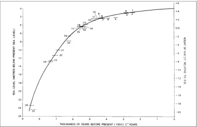
1976; Shennan and Horton, 2002), as shown in Figure 1.2.
Allen (2000c) argues that this broad, smooth curve is a misleading representation of
Holocene sea-level change in the region, depicting only the underlying behaviour of sea-level
and potentially masking the existence of centennial scale, decimetre to metre-scale variation
in the record. Subsequent work at Gordano by Hillet al.(2007) reveals that marine influence
in this part of the Severn Estuary was not uniform throughout the Holocene, but it is not
possible to infer whether such changes in marine influence were due to sea-level changes given
the magnitude of error in the chronolgical and geological records.
Heyworth and Kidson (1982) argued that any possible oscillations in sea-level would
probably be of a lesser magnitude than the vertical errors associated with studies of RSL
change. However, improved knowledge and more robust and precise methods may now mean
2Note the two spellings of Steart/Stert forSteart village,Steart Peninsula,Stert Flats, Stert Point and
Chapter 1. Introduction 6
Somerset Levels and Moors Steart Peninsula
M EN
D IP H
ILLS
QU AN
[image:20.595.114.552.55.492.2]TOC K HILLS
Figure 1.1: Map of the Severn Estuary levels, showing places mentioned in the text. Adapted from Allen and Haslett (2002) with permission from SAGE Publications.
that fluctuations in the direction and rate of Holocene sea-level change can be reflected in
the reconstruction of regional RSL.
Many of the data points in Kidson and Heyworth’s sea-level curve for the Bristol Channel
region are from Bridgwater Bay (Kidson and Heyworth, 1976). While this research is
signif-icant and has been influential, it is of its time. The methods used to compile the sea-level
curve are not sufficiently rigorous by the research standards of the present day, and have
since been criticised by Allen (2000c) and Haslett et al. (1998). These criticisms are based
around a lack of acknowledgement that the relationships between the peat units selected for
SLIPs and past sea-levels are unknown. These data points have been used in a meta-analysis
of relative land/sea-level change in the British Isles by Shennan and Horton (2002) without
Figure 1.2: Holocene sea-level rise in the Bristol Channel, from Kidson and Heyworth (1976). Dates are in 14C years and numbers on the plot refer to sea-level index points presented in the publication. Reproduced with permission from The Geological Society of London.
This thesis presents a transfer-function derived sea-level history for the Steart Peninsula,
examines the relative merits of single- and multi-proxy transfer functions, and places this
new sea-level reconstruction in the context of Holocene sea-level and environmental change
in the wider and Severn Estuary region.
1.3 Thesis aims and objectives
The aims of this thesis, and the objectives set out in order to address those aims, are as
follows:
Aim 1: To develop single- and multi-proxy sea-level transfer functions for the macrotidal
Severn Estuary region
(a) To establish the key environmental factors affecting the presence and species abundance of surface-dwelling intertidal diatoms and foraminifera in the contemporary Severn
Estuary intertidal zone.
(b) To develop single- and multi-proxy sea-level transfer functions based on the relationships between species and mean tidal level (MTL).
Chapter 1. Introduction 8
Aim 2: To reconstruct Holocene sea-level at the Steart Peninsula, Somerset.
(a) To apply the preferred sea-level transfer function to fossil microfaunal assemblages from a dated sediment sequence from the Steart Peninsula.
(b) To integrate the transfer function-derived sea-level history into the existing understand-ing of Holocene sea-level and environmental change in Bridgwater Bay and the wider
Severn Estuary region.
Aim 3: To provide a critical reflection of the quantitative methodology used and make
methodological recommendations for the use of multi-proxy transfer functions in the
Sea-Level Variability and
Reconstruction
This chapter provides reviews of the literature on Holocene sea-level change and
reconstruc-tion, with a particular focus on biological sea-level indicators and quantitative methods, and
explores the evolution of methods since the mid-twentieth century.
Following a brief introduction to Quaternary science and sea-level research, some key
terms used in sea-level studies are defined, and literature on sea-level indicators, qualitative
and quantitative sea-level reconstruction and the particular problems posed by macrotidal
estuaries are considered in order to inform the thesis aims and objectives. Literature specific
to the geographical region of this study can be found in Chapter 3.
2.1 Quaternary climate and sea-level variability
The total global volume of ocean water (O) is a function of the total water in the Earth
system and the various stores of water on-land. Rearranging the equation for the global
hydrological balance of Pirazzoli (1996, p. 6) for O gives the following:
O =K−A−L−R−M−B−S−U−I (2.1)
Where:
• O = oceans and seas
• K= global water (constant)
• A = atmospheric water
• L = lakes and reservoirs
Chapter 2. Sea-Level Variability and Reconstruction 10
• R = rivers and channels
• M = soil moisture
• B = biological water
• S = swamps
• U = ground water
• I = frozen water
Pirazzoli (1996) estimates that A, R, S, B and M together represent only 24cm of global
sea-level, implicating lakes, reservoirs, ground water and land-based ice as the greatest
poten-tial contributors to ocean water volume. Indeed, the main factor influencing global sea-level
during the Quaternary period has been the climatic forcing that causes contintenal ice sheets
to increase and decrease in volume according to changes in insolation (Wilsonet al., 2000).
The Quaternary period began approximately 2.6 million years BP and continues today
(Mascarelli, 2009). Broadly speaking, the Quaternary climate has oscillated between long
glacial (90,000 to 100,000 years) and shorter interglacial (10,000 to 15,000 years) episodes with
a c. 100,000 year periodicity controlled by astronomical forcing. The present interglacial, in
which the human population has expanded significantly, is the Holocene. A 100,000 year cycle
is more prominent in records of the last one million years (Bradley, 1999), perhaps suggesting
that variation in the eccentricity of the earth’s orbit around the sun is an important climate
forcer during this time. However, Milankovitch theory (Hays et al., 1976) indicates a shift
away from the prominence of eccentricity at a 100,000 year periodicity in the last one million
years, and an increase in variance at lower frequencies (∼400,000 years). It is probable
that the observed 100,000 year periodicity results from feedbacks within the climate system,
amplifying the underlying orbital pacemaker of eccentricity (Bradley, 1999).
When ice sheets expand during glacials ocean water is enriched in the heavier stable
oxygen isotope18O. This enrichment is recorded in the preserved calcium carbonate (CaCO3)
tests of benthic marine microorganisms such as foraminifera. The glacial and interglacial
periods in the Earth’s climatic history are thus referred to as marine isotope stages (MIS),
based on the stable oxygen isotope record (δ18O) obtained from deep sea cores (Emiliani,
1955). The Holocene is MIS 1 and the last glacial is MIS 2. The preceding Quaternary glacial
cycles are numbered chronologically in this way, with odd numbers denoting interglacials and
concentration of data used in the LR04 stack is at least twice
as high as in any previous stack or individuald18O record
spanning that interval. The stack’s resolution is comparable to previous stacks but is less than half that of the highest-resolution records.
[17] The LR04 stack is simply the average of the aligned
benthicd18O records. We do not adjust the mean or variance
of the records, except to make species offset corrections. We choose not to adjust the isotope curves based on their modern bottom water temperatures because the temperature differences between sites may have changed dramatically over the last 5.3 Myr. We also do not weight the records based on their spatial distribution. The majority of records are from the Atlantic Ocean, and the number of sites in the stack varies with time, changing the relative weighting of different regions. However, we observe that regional
differ-ences in benthicd18O are typically less than 0.3%(less than
0.15%after 0.6 Ma), and we are currently developing a
detailed description of regionald18O variability.
5. Age Model
[18] Because the LR04 stack is constructed by graphic
correlation, its stratigraphic features are essentially inde-pendent of any timescale. Below we describe the con-struction of an age model which takes advantage of the high signal-to-noise ratio of the stack and analysis of the sedimentation rates at 57 sites. However, almost any age model could be applied to the LR04 stack. This flexibility
allows the stack to be adapted to alternate models ofd18O
response or to improvements in age estimates.
[19] We construct the LR04 age model by aligning our
benthicd18O stack to a simple model of ice volume while
considering the average (stacked) sedimentation rate of
Figure 4. The LR04 benthicd18O stack constructed by the graphic correlation of 57 globally distributed
benthicd18O records. The stack is plotted using the LR04 age model described in section 5 and with new
MIS labels for the early Pliocene (section 6.2). Note that the scale of the vertical axis changes across panels.
[image:25.595.113.551.57.281.2]6 of 17
Figure 2.1: Stacked Quaternary δ18O record for the last 3.6 million years constructed by the
graphic correlation of 57 globally distributed, individual benthicδ18O records. The horizontal axis is time in thousands of years. Note that the scale of the vertical axis changes across the panels. Adapted from Lisiecki and Raymo (2005) with permission from John Wiley and Sons.
Since theδ18O record relates closely to the volume of water that is locked up in continental
ice, it follows that that same record should have a relationship with global sea-level. However,
Chappell and Shackleton (1986) and Shackleton (1987) have shown that the relationship
between δ18O record and sea-level is complex and may not have been constant over time.
Theδ18O of benthic foraminifera may not only have been influenced by oceanicδ18O over the
Quaternary, but also by deep ocean temperature and salinity (Wilson et al., 2000). If either
one of these has varied during the Quaternary the ability of the δ18O record to produce a
reliable global sea-level record is compromised. However, a comparison of the δ18O record
with a eustatic sea-level curve derived from a series of raised coral terraces on the Huon
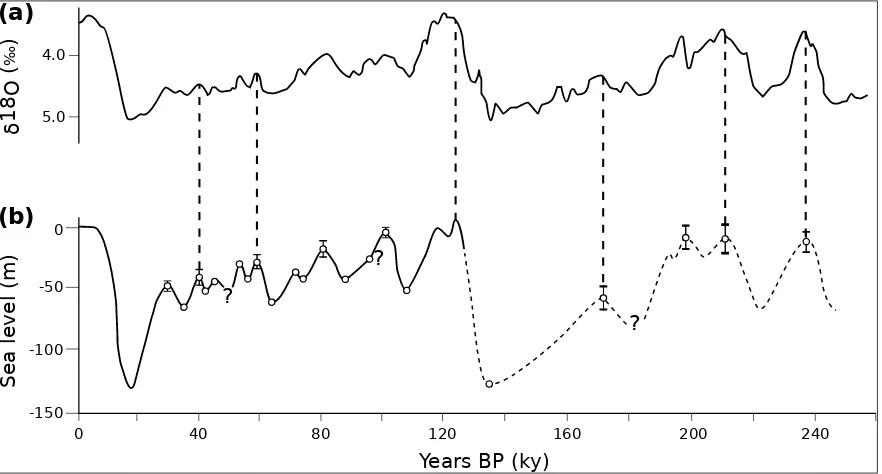
Peninsula, New Guinea (see Figure 2.2) indicates that δ18O is still a good general
proxy-indicator of Quaternary sea-level (Masselink and Hughes, 2003).
The coral terrace-derived sea-level curve from the Huon Peninsula (Figure 2.2)
demon-strates the magnitude of the vertical change in sea-level that occurs from interglacial to glacial
periods. For example, the LGM was accompanied by a sea-level lowstand of ∼140m below
present mean sea-level (MSL) (Chappell and Shackleton, 1986), providing the base level
dic-tating the lower limit of the occurrence of subaerial erosion processes such as fluvial erosion.
The rivers of the Severn Estuary region cut deep valleys into the land surface when
Pleis-tocene sea-level was low, and these valleys were later infilled with Holocene sediments under
Chapter 2. Sea-Level Variability and Reconstruction 12
4.0
5.0
0
-50
-100
-150
0 40 80 120 160 200 240
Years BP (ky) (a)
(b)
Sea level (m)
δ
18
O
(
‰
)
? ?
[image:26.595.114.555.56.293.2]? ?
Figure 2.2: Correspondence between (a)δ18O record from east equatorial core V19-30, from measurements of benthic Uvigerina senticosa and (b) eustatic sea-level curve for the Huon Peninsula, New Guinea, over the last 250,000 years. Adapted from Chappell and Shackleton (1986) by Masselink and Hughes (2003). Reproduced with permission from Taylor & Francis.
history of the Severn Estuary region is discussed further in Chapter 3.
2.2 Holocene climate and sea-level variability
The Holocene epoch denotes the Earth’s current interglacial climate. The LGM of the British
and Irish Ice Sheet (BIIS) occurred about 22,000 years BP, based on recent evidence from
36Cl surface-exposure dating, amino acid geochronology of marine shells in glacial deposits
and AMS radiocarbon dating (Bowenet al., 2002). The termination of the most recent glacial
(MIS2), in which glacial conditions gave way to Holocene climate, began around 14,500 years
BP (Walkeret al., 2009).
The transition of the Earth’s climatic mode from the LGM to the start of the Holocene
is well-studied. This LGM-Holocene period is relatively recent, with respect to the wider
Quaternary period and the rest of the Earth’s history, and much evidence for environmental
change is readily available in sedimentary, archaeological, marine and other records. This
period represents a ‘case-study’ of large, centennial-scale changes in global climate, and more
specifically of the rising global mean surface temperature (GMST) (Oldfield, 2005; PALSEA,
2009). Sea-level researchers are interested in this post-LGM period of warming, because
improving our understanding of the responses of ice sheets, glaciers and thermal expansion
of the oceans to warming during this time will help to constrain the likely contribution of
The most recent proposal for the official date of the onset of the Holocene comes from
the NGRIP and is defined in the ice core record as the horizon which shows the clearest
signal of climatic warming, marked by a step change in deuterium values (Walker et al.,
2009). Walker et al. (2009) proposed 11,700 years BP as the new Global Stratotype Section
and Point (GSSP) for the Pleistocene-Holocene boundary. The transition from glacial to
interglacial climate in the Northern Hemisphere was not continuous or uni-directional and
was interrupted initially between 12,900 and 11,500 years BP by a short-lived cold event
known as the Younger Dryas or Greenland Stadial 1.
There is evidence for a further oscillation in climatic warming in the North Atlantic at
around 8,200 years BP that lasted about 160 years (Schmidt and Jansen, 2006). This sudden
cold event is known as the ‘8.2kyr event’ and has been identified in theδ18O record from the
Greenland Ice Sheet Project 2 (GISP2), the Greenland Ice Core Project (GRIP) and NGRIP
ice cores (Rohling and Palike, 2005), and in other proxy records (Nesje and Dahl, 2001).
The cooling event is attributed to a slowdown in the North Atlantic Deep Water formation
following an outflow of meltwater into the North Atlantic from the Lakes Agassiz and Ojibway
(Kendallet al., 2008). This rapid meltwater pulse raised global sea-level abruptly and recent
research in the Netherlands supports a possible multi-staged lake drainage and, given the
distance of the study site from the Laurentide proglacial lakes, a global sea-level event of
greater magnitude than previous estimates (3.0±1.2m versus 0.4-1.4m) (Hijma and Cohen,
2010)
The post-glacial contraction of continental ice sheet coverage caused rapid global
sea-level rise of about 130m between the LGM and ∼6,000 years BP. Since then, about 10m of
global sea-level rise has occurred, representing relative stability in global sea-level since the
mid-Holocene (Haslett, 2000).
The term ‘eustatic’ is often used to refer to absolute sea-level change, or global change,
such as an increase or decrease in ocean water volume, that is independent of regional
vari-ation. In the 1960s researchers attempted to compile a global Holocene eustatic sea-level
curve based on work by Godwinet al.(1958) on low-lying parts of the British Isles and work
by Fairbridge (1961) in other parts of the world. It was at this point, when the ‘eustatic’
sea-level curve appeared to contain many sequences of oscillations, that it became apparent
to the sea-level community that the pattern and timing of Holocene sea-level change was not
uniform across the planet. There is little controversy around the broad shape of postglacial
sea-level rise, with most of the sea-level community agreeing on something like the curve
Chapter 2. Sea-Level Variability and Reconstruction 14
(Masselink and Hughes, 2003). The term ‘ice-equivalent’ is now more often used in place of
‘eustastic’, which is itself now more a concept than an observable entity (Gehrels, 2010).
Gehrels (2010) outlines a debate over the timing of the final contribution of ice melt to
the oceans in the mid- to late-Holocene, with estimates ranging from 6,000 years BP (Bassett
et al., 2005; Morhange and Pirazzoli, 2005) to 5,000 years BP (Milneet al., 2005), 4,000 years
BP (Peltier, 1998, 2002; Peltieret al., 2002) and as recent as 1,000 years BP (Fleming et al.,
1998). The IPCC’s Fifth Assessment Report concludes that it is likely that the global ocean
water volume increased by 2 to 3m between 7,000 and 3,000 yearsBP (Masson-Delmotteet al.,
2013) and that in the last 2,000 years global MSL has not fluctuated by more than ±0.25m
over timescales of several hundreds of years (Church et al., 2013). The exact timing of the
end of ice-melt contribution to the global oceans has still not been resolved, but significant
[image:28.595.215.446.353.657.2]progress has been made since the IPCC’s fourth assessment report (Churchet al., 2013).
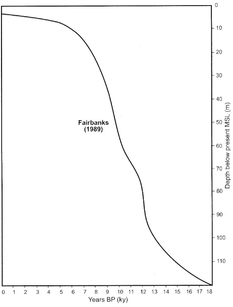
Figure 2.3: Eustatic sea-level curve for the Holocene, adapted from Fairbanks (1989) by Masselink and Hughes (2003) and reproduced with permission from Taylor & Francis.
Relative sea-level refers to the level of the sea relative to the land on a regional scale,
and change can be due to a combination of ocean water volume variation and vertical land
movement (Masselink and Hughes, 2003). Glacio-isostatic adjustment in and close to deglacial
1998). In the British Isles, while eustatic change over the Holocene has been one of sea-level
rise, the isostatic effects following the termination of the last glacial mean that the Northern
part of the British Isles is experiencing slight relative sea-level fall where rebound occurs from
the former loading of the BIIS, while relative sea-level is rising in the South as the glacial
forebulge collapses (Peltier, 1998; Shennan and Horton, 2002).
Pethick (1984) argues that we should be most concerned with relative sea-level change,
since that is what ultimately affects coastal areas, ecological habitats and human populations,
and because the effect in terms of coastal morphology is similar whether a sea-level rise is
the result of an isostatic fall in the level of the land or an eustatic rise in sea-level. However
the Woodroffe and Murray-Wallace (2012) highlight the importance of the detection of a
global, eustatic element to sea-level change, in order to quantify that which is attributable
to thermal expansion and additional meltwater to the oceans, resulting from the greenhouse
effec. The IPCC’s Fifth Assessment report emphasises progress in monitoringglobal MSL rise
in the 21st century as well as developments in observing regional sea-level changes (Church
et al., 2013) and in the use of palaeoclimatic archives in modelling climatic warming and
establishing a Holocene baseline for the discussion of anthropogenic contributions to climatic
and sea-level change (Masson-Delmotteet al., 2013).
2.3 Sea-level indicators
Many sedimentary and geological records contain evidence of former sea-levels, some of which
can be dated, providing the information with which to construct regional sea-level histories.
The modern coastal environment and the behaviours of the waves, tides and coastal
sedi-ments and biota that we can study today provide a wealth of information that can be used to
infer meaning from fossil sedimentary deposits, archaeological remains and erosional features
(Pirazzoli, 1996). Kemp et al. (2012, p. 26) define a sea-level indicator as “. . . a physical,
biological or chemical feature possessing a systematic and quantifiable relationship to
eleva-tion in the tidal frame”. This seceleva-tion discusses some of the methods used to infer meaning
from sea-level indicators in the following three categories: geomorphological, archaeological
and biological. Sea-level indicators in these categories are often used in combination with
one another in studies of former sea-level change (Faivre et al., 2013).
2.3.1 Geomorphological sea-level indicators
Geomorphological indicators of sea-level can be erosional or depositional features (Haslett,
Chapter 2. Sea-Level Variability and Reconstruction 16
in hard rock (Pirazzoli, 1996), while depositional indicators include features such as fossil
beaches, saltmarshes and tidal flats (Lambeck et al., 2010). A good understanding of the
processes by which morphological features have been formed is a key factor in using them as
sea-level indicators (Pirazzoli, 1996).
An important example of a depositional geomorphological sea-level indicator in the Severn
Estuary region is the Burtle Formation, which includes shelly marine sands and gravels of the
Kenn Church Member (formerly the Burtle Beds of Bulleid and Jackson (1937)) (Campbell
et al., 1999). These mostly marine shelly sands are raised in the order of tens of metres
above the alluvial deposits of the Somerset Levels and are thought to relate to at least
two interglacials, MIS 5e and MIS 7 (Campbell et al., 1999). The Burtle Beds provide an
example of a landform that is composed of more than one type of sea-level indicator. While
the raised beds themselves would be classed as depositional indicators, the bivalve shells and
foraminifera and ostracod tests found within them provide biological evidence for the former
sea-levels (Hunt, 2006).
Depositional features indicating lower former sea-levels include fossil saltmarsh peats,
buried by marine or estuarine silts and clays under a transgressive sea-level regime (Masselink
and Hughes, 2003). Peats are organic and can be dated using radiometric dating techniques
such as 14C for sediments up to ∼60,000 years old and210Pb for peats deposited in the last
∼100 years (Gehrels, 2000; Leorri et al., 2006). Kidson and Heyworth (1976) used buried
peats as sea-level indicators to produce their Holocene sea-level curve for Bridgwater Bay.
Today it is standard practice to combine stratigraphic work such as this with the study
of the biological indicators (for example pollen, diatoms and foraminifera) preserved within
the peats. This approach is discussed in more detail below, following a brief discussion of
archaeological sea-level indicators.
2.3.2 Archaeological sea-level indicators
Effective examples of archaeological evidence for sea-level change can be found in various
locations around the world, but most commonly in the Mediterranean, where human activity
is recorded as far back as the LGM (Lambecket al., 2010). Archaeological evidence of to
sea-level changes will generally be one of two types; structures with no specific former relationship
with sea-level, such as dwellings built on the land and since flooded by the sea, and those such
as slipways, fish tanks and harbours that were constructed in the past specifically in order to
exploit a particular relationship with tidal-level and might no longer function today due to a
evidence in the form of fish tanks with modern data on tidal levels to estimate changes in
sea-level at the Tyrrhenian coast of Calabria in Italy from 1,806 years BP onwards.
The one clear limitation of archaeological evidence is its location-specific nature. A piece
of archaeological evidence found and studied in isolation can only offer insight into a change in
sea-level in a strictly local context. Other limitations include the exclusion of structures built
on unstable land surfaces, the uncertain use of some ancient structures, and the uncertain
relationship that many structures have with sea-level (Lambecket al., 2010). The submerged
remains of a dwelling clearly indicate a marine incursion but do not necessarily indicate the
magnitude of sea-level rise. Archaeological evidence can therefore lack accuracy and precision
(Pirazzoli, 2005). However, archaeological evidence may be used in conjunction with other
categories of sea-level indicator. For example, there may be biological organisms preserved
upon the surface of an ancient structure that can be cross-referenced with modern equivalents
with reference to elevation relative to mean sea-level (Morhange et al., 2001). Investigating
two lines of enquiry can often increase the reliability of a reconstruction. Archaeological
in-dicators may also be used in combination with historical data. Although historical accounts
of past events or environments will not meet the rigorous modern criteria of scientific
mea-surement, qualitative information can certainly contribute to the reconstruction of regional
sea-level change over previous decades and centuries (Pirazzoli, 1996). For example, ancient
writers such as Columella explained how marine fishtanks were constructed in the
Mediter-ranean in the first centuryad, and what their relationships with tidal levels were (Pirazzoli,
1988).
Researchers have been conducting an extensive programme of archaeolgical investigation
of the Severn Estuary Levels since the 1980s (Bell, 1993, 1994; Bell and Neumann, 1997;
Bell et al., 2003; Walker et al., 1998). Finds have included human and animal footprints,
human skulls, remains of buildings, wooden trackways, pottery and wooden posts, dating
from the Mesolithic to post-Medieval times. Of particular relevance to sea-level research
are the Somerset Levels trackways, likely to have been constructed to sustain contact across
communities in wet areas (Bell and Neumann, 1997), a line of stakes thought to be fish traps
at Gore Sand (Nayling, 2002), and fossilised drainage channels along with mid-3rd century
pottery that suggests that extensive drainage took place at an eroded Roman settlement
on the Wentlooge Levels in South Wales (Allen and Fulford, 1986; Fulford et al., 1994).
Discussion of the wooden trackways and of the debates around the possibility of a marine
transgression in the Roman Era can be found later in Section 3.5 of Chapter 3.
mod-Chapter 2. Sea-Level Variability and Reconstruction 18
ern characteristics, but this is not always possible with archaeological indicators.
Further-more, while it might be possible to date an artefact and infer something about its use, its
relationship with sea-level might not be clear, and nor may it be possible to know whether
an item was buried, and if so, how deep, or if it was transported post-deposition (Nayling,
2002). Nevertheless, archaeological indicators contribute important information to studies
of Quaternary sea-level and one of the aims of IGCP588 (Preparing for Coastal Change) is
to embrace interdisciplinary research so that archaeology in coastal areas might contribute
more to sea-level research as well as to our understanding of the social and cultural aspects
of past societies (Switzeret al., 2012).
2.3.3 Biological sea-level indicators
Living organisms that exist at known tidal ranges, and that can become stranded or buried
by changes in sea-level, often occupy narrow vertical ranges (Lambecket al., 2010) and can be
used to document these changes. Biological sea-level indicators are some of the most accurate,
and organisms can include those, like barnacles and mussels, that adhere to hard surfaces
such as rocky cliffs and sea walls, and those that inhabit intertidal sediments (Masselink
and Hughes, 2003). The latter tends to consist of microscopic organisms that are often
fossilised in coastal sediments, as well as fossil pollen and plant macrofossils produced by
coastal vegetation, that can indicate former changes in salinity and thus the position of the
local water level (Pirazzoli, 1996).
In tropical waters the rates of growth in coral reefs are known to be governed mainly
by water temperature and water depth, the latter often being directly related to MSL, and
some species produce annual or seasonal bands that have allowed, in some cases, for detailed
sea-level histories and marine conditions to be documented (Lowe and Walker, 1997).
The geographical research focus is dominated by a large estuary whose waters have
de-posited an archive of Holocene sediments upon the land over the past ∼12,000 years (Allen
and Rae, 1987). The tidally-dominated estuary is characterised by the prevalence of
salt-marshes and tidal flats whose sediments are inhabited by tide-dependent microorganisms
(see Chapter 3). For this reason, the focus of the remainder of this section is on the
bio-logical indicators that inhabit contemporary intertidal sediments and are preserved in the
region’s Holocene sedimentary sequences.
i Foraminifera as sea-level indicators
Forming the order Foraminiferida in the phylum Protista, a foraminifer is described by
more interconnected chambers.” Foraminifera are single-celled organisms, and each of the c.
10,000 modern species can be classified by its form and test composition. Benthic forms live
on the sea floor (Murray, 1991a) while planktonic species live within the water column
(Mur-ray, 1991b). Tests may be agglutinated (made of detrital sediment particles held together
with cement), porcellaneous (calcareous with translucent walls) or hyaline (calcareous with
glassy, transparent shells) (Murray, 2002).
All intertidal foraminifera that are used as sea-level indicators are benthic, living in or just
below the sediment surface (Gehrels, 2002). Saltmarsh foraminifera are mainly agglutinated
and are able to withstand the relatively acidic saltmarsh conditions, while tidal flat and tidal
creek taxa are mainly those with calcareous tests (Gehrels, 2002).
Foraminifera are effective tidal indicators for a number of reasons. They exhibit strong
correlation with elevation above mean sea-level (Scott and Medioli, 1978), are well preserved
and straightforward to detect in accumulated saltmarsh sediments and often occur in large
quantities (Horton and Edwards, 2006).
Pioneering work by Scott (1976) and Scott and Medioli (1978, 1980, 1986) changed the
way that sea-level reconstruction has been attempted in recent decades. Scott (1976) and
Scott and Medioli (1978) showed that foraminifera are organised into well defined zones in
the modern intertidal sediments in Southern California, USA and Chezzetcook Inlet in Nova
Scotia, Canada, meaning that rather than continuing to arbitrarily equate fossil saltmarsh
sediments to a fixed altitude, it became common practice to subdivide fossil deposits into these
zones, thereby increasing the potential vertical resolution of sea-level reconstructions. The
authors found that the east and west coasts of the North American continent showed sim