The interaction between equity and credit risks

(1)

THE INTERACTION BETWEEN

EQUITY AND CREDIT RISKS

Amer Demirovic

A thesis submitted in partial fulfilment of the requirements of

the University of the West of England, Bristol

for the degree of Doctor of Philosophy

Bristol Business School

University of the West of England

Bristol

(2)

This copy has been supplied on the understanding that it is copyright material

and that no quotation from the thesis may be published without proper

(3)

(4)

Acknowledgments

The completion of a PhD thesis is always a great challenge. Doing it on a part-time

basis, and away from the campus seems almost impossible. In my case, it would have

been very difficult for me to complete this work without the support and flexibility

of my supervisors, Professor Jon Tucker and Professor Cherif Guermat. They greatly

helped me throughout the entire process, from the collection of data, through the

development of empirical models, to the formulation of conclusions. As if that was

not enough, they recommended me for the UWE Completion Bursary which enabled

me to attend UWE for two months and speed up the completion of the thesis by at

least a year. I am also thankful to UWE for awarding me the bursary, and to Dr.

Helen Frisby and the friendly staff at the Graduate School Office for superbly

administering the entire process.

A full-time job and a part-time PhD leaves you no time for anyone else. For this, I

would like to express my gratitude to my family for their unconditional support; my

girlfriend Azra (who has become a wife during the process) for managing to stay with

me during these four years and actually helping by adding references to RefWorks;

my close friends for remaining close friends despite having barely seen me over

these last four years; my colleagues at the HJPC BiH for doing my job during my

leaves to attend UWE; and last but certainly not the least my friend, Ermin Mulabdic,

(5)

Abstract

Equity anddebt are two distinct classes of securities in terms of investing risks and potential return, buttheir value depends on the same underlying assets of the firm and therefore the risk-return tradeoff of each security should be systematically

related. Following a review of the principal theoretical approaches to the

measurement of equity and credit risks,this thesis utilizes a sample of matched firm-level equity and corporate bond data to examine three aspects of risk interaction. First, it investigates the importance of idiosyncratic and systematic equity risks in determining the credit spread on corporate bonds. Second, the thesis investigates how equity and credit risks themselves impact upon the correlation between equity and bond returns. Finally, the thesis examines whether the credit sensitive information contained within financial accounting data is fully reflected in equity prices. The empirical approach adopted in this thesis is to relate the credit spread and the conditional correlation between equity and bond returns with both equity and credit risk indicators and financial accounting variables. This methodological approach enables an extension of the existing literature on several dimensions, leading to a number of empirical results which have important theoretical and practical implications for the integrated management of equity and credit risks. Consistent with existing empirical studies, equity and credit risks are found to exert a positive impact upon the credit spread. Surprisingly, equity volatility is found to significantly outperform the distance to default in terms of explanatory power.

Further, the impact of equity volatility increases monotonically as the distance to default narrows. The conditional correlation between equity and bond returns is found on average to be positive and to vary over time, peaking during the 2007

financial crisis. Finally, an increase in credit risk has a positive impact upon the

correlation while an increase in equity risk is found to strengthen the correlation only

(6)

CHAPTER 1 ... 1

1.1. Introduction... 1

1.2. Background and Rationale ... 2

1.3. Objectives and Contributions of the Thesis ... 4

1.4. Structure of the Thesis ... 5

1.5. Methodological Considerations ... 6

1.5.1. Equity Risk ... 6

1.5.2. Credit Risk ... 7

1.5.3. Regression Analysis ... 7

1.6. Main Research Questions ... 8

CHAPTER 2 ... 9

2.2. The Structural Approach ... 10

2.3. Limitations of the Structural Approach ... 14

2.4. Estimation of the Structural Model ... 15

2.4.1. Estimating Unobservable Value of Firm’s Assets and the Volatility of Assets ... 15

2.4.2. Choosing Default Point and Time Horizon ... 19

2.4.3. Estimating the Expected Growth in the Assets Value ... 21

2.5. Extensions of the Structural Model ... 22

2.5.1. Early Default ... 23

2.5.2. Stochastic Interest Rate ... 25

2.5.3. Stochastic Default Barrier... 28

2.5.4. Mean-Reverting Leverage Ratio ... 30

2.5.5. Jump Diffusion ... 31

2.5.6. Stochastic Volatility ... 32

2.5.7. Endogenous Default Barrier ... 33

2.6. Summary ... 34

CHAPTER 3 ... 36

3.2. A Basic Model for Equity Prices ... 36

3.3. Equity Risk and Return Trade-Off ... 38

3.4. Equity Value Determinants ... 41

3.4.1. Capital Assets Pricing Model ... 41

3.4.2. Multi-Factor Models ... 46

3.5. The Equity Premium ... 54

3.5.1. Equity Premium Determinants ... 55

3.5.2. Time Variation of the Equity Premium and its Implications ... 57

3.5.3. Estimation of the Equity Premium ... 60

3.6. Equity Volatility ... 62

3.6.1. Estimation of the Equity Volatility ... 62

3.6.2. Volatility Components ... 67

(7)

CHAPTER 4 ... 72

4.2. Literature Review and Development of Hypotheses ... 74

4.2.1. Relationship between the Credit Spread and Equity Volatility ... 75

4.2.2. Relationship between the Credit Spread and Distance to Default ... 77

4.2.3. Systematic and Idiosyncratic Equity Risks as Determinants of Credit Risk ... 78

4.2.4. Interaction between Equity Volatility and the Distance to Default ... 80

4.2.5. Relationship between the Credit Spread and Common Factors ... 81

4.3. Methodology ... 83

4.3.1. Credit Spread ... 83

4.3.2. Bond Issue Characteristics ... 85

4.3.3. Equity Volatility ... 85

4.3.4. Equity Returns ... 86

4.3.5. Distance to Default ... 88

4.3.6. Panel Data Analysis ... 89

4.4. Data ... 91

4.5. Summary ... 96

CHAPTER 5 ... 98

5.2. The Relationship between the Credit Spread and Equity Volatility ... 99

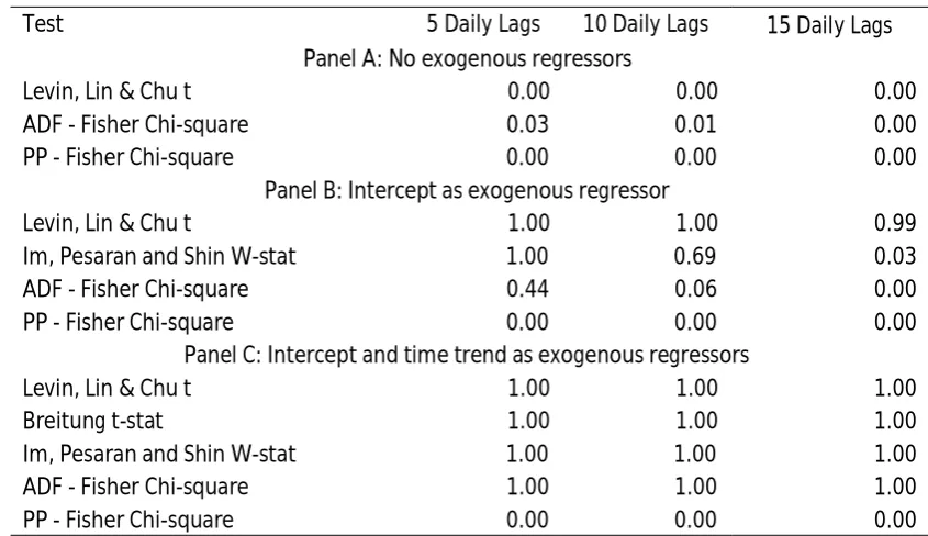
5.2.1. Unit Root Analysis ... 99

5.2.2. The Constant Coefficient Model ... 100

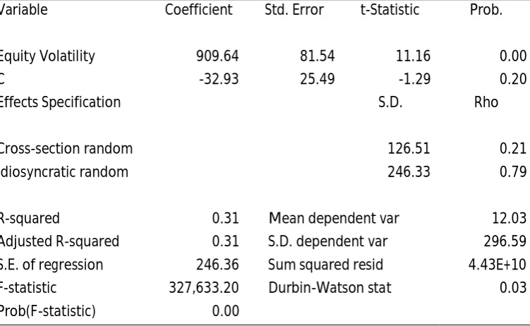
5.2.3. The Cross-sectional Fixed Effects Model... 103

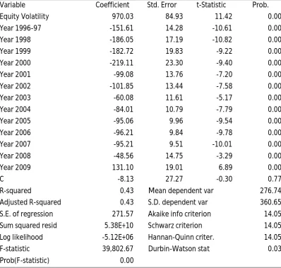
5.2.4. The Period Fixed Effects Model ... 106

5.2.5. The Two-way Fixed Effects Model ... 110

5.3. The Relationship between the Credit Spread and the Distance to Default of Merton (1974) ... 112

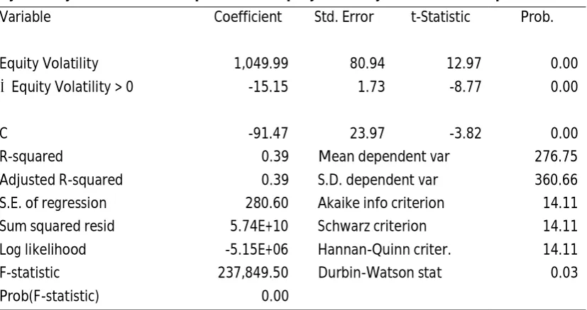
5.4. Systematic and Idiosyncratic Equity Volatility as Determinants of the Credit Spread... 119

5.5. The Interaction between Equity Volatility and Credit Risk in Explaining Variations in the Credit Spread ... 126

5.6. The Relationship between the Credit Spread and Common Factors ... 130

5.7. Changes in the Credit Spread ... 137

5.8. Robustness of the Results ... 139

5.8.1. Equity Volatility Modelled as an Asymmetric EGARCH Process ... 139

5.8.2. Firm Size ... 140

5.8.3. Bond-specific Variables ... 142

5.9. Summary ... 144

CHAPTER 6 ... 149

(8)

6.2.2. Equity Volatility and the Correlation between Equity and Bond

Returns ... 153

6.2.3. Credit Risk and the Correlation between Equity and Bond Returns .... 154

6.2.4. Interaction between Equity Volatility and the Distance to Default ... 156

6.2.5. Common Factors and the Correlation between the Equity and Bond Returns ... 157

6.3. Methodology ... 160

6.3.1. Equity and Bond Returns ... 160

6.3.2. Conditional Correlation between the Equity and Bond Returns ... 160

6.3.3. Equity Volatility ... 162

6.3.4. Distance to Default ... 163

6.3.5. Equity Systematic Returns and Volatility ... 163

6.3.6. Bond Issue Characteristics ... 164

6.4. Data ... 166

6.5. Summary ... 167

CHAPTER 7 ... 169

7.2. The Conditional Correlation between the Equity and Bond Returns ... 170

7.3. The Relationship between Equity Volatility and the Correlation between the Equity and Bond Returns ... 173

7.4. The Relationship between the Distance to Default of Merton (1974) and the Correlation between the Equity and Bond Returns ... 178

7.4.1. The Constant Coefficient model ... 178

7.5. The Interaction between the Equity Volatility and Credit Risk in Explaining Variations in the Correlation between the Equity and Bond Returns ... 183

7.6. The Relationship between Common Factors and the Correlation between the Equity and Bond Returns ... 186

7.7.1. The Correlation between the Equity and Bond Returns Modelled as an Asymmetric Diagonal VECH Process ... 190

7.7.2. The Firm Size ... 191

7.7.3. Bond-specific Variables ... 192

7.8. Summary ... 194

CHAPTER 8 ... 199

8.2.1. Accounting-based Indicators of Credit Risk ... 200

8.2.2. Comparing the Impact of Accounting and Market based Measures on the Credit Spread ... 203

8.2.3. The Incremental Information Value of Financial Accounting Data ... 204

(9)

8.3.1. Credit Spread and Bond Characteristics ... 206

8.3.2. Accounting Variables... 207

8.3.3. Market-based Variables ... 209

8.4. Data ... 211

8.5. Summary ... 213

CHAPTER 9 ... 216

9.2. The Correlation between the Financial Accounting Ratios and the Credit Spread ... 217

9.3. The Relevance of Financial Accounting Variables in the Measurement of the Credit Spread ... 219

9.4. The Relevance of Equity Market-based Indicators of Credit Risk in the Measurement of the Credit Spread ... 229

9.5. The Incremental Relevance of Financial Accounting Variables in the Measurement of the Credit Spread ... 238

9.7. Summary ... 248

CHAPTER 10 ... 252

10.1. Introduction ... 252

10.2. Main Findings and Contributions ... 253

10.2.1. The measurement of credit risk ... 253

10.2.2. The measurement of equity risk ... 255

10.2.3. Empirical findings ... 256

10.3. Limitations of the Thesis ... 264

10.4. Further Research ... 265

References ... 267

(10)

List of Tables

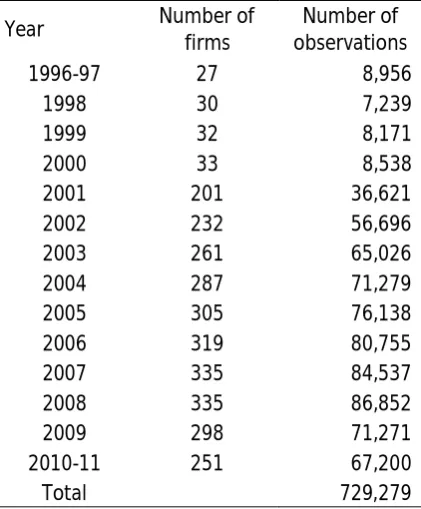
Table 4.1. Number of firms and observations in the sample ... 93

Table 4.2. Descriptive statistics of the data series ... 93 Table 5.1. Probability values of panel unit-root tests for the credit spread ... 100

Table 5.2. The relationship between equity volatility and the credit spread:

the constant coefficient model ... 101 Table 5.3. A panel unit-root test analysis of the residuals from regressing the

credit spread on equity volatility ... 102

Table 5.4. Asymmetry in the relationship between equity volatility and the

credit spread ... 103

the cross-sectional fixed effects model ... 104 Table 5.6. Redundant fixed-effects tests ... 105

the cross-sectional random effects model ... 106 Table 5.8. Test of random-effects specification ... 106

the period fixed effects model... 108 Table 5.10. The relationship between equity volatility and the credit spread

within the time sub-samples ... 109

the two-way fixed effects model ... 111 Table 5.12. The relationship between the distance to default and the credit

spread: the constant coefficient model ... 112

Table 5.13. Panel unit-root test analysis of residuals from regressing the credit spread on the distance to default ... 113 Table 5.14. The relationship between the distance to default and the credit

spread: the cross-sectional fixed effects model ... 114 Table 5.15. Redundant fixed-effects tests ... 115

Table 5.16. The relationship between the distance to default and the credit

spread: the period fixed effects model ... 116

spread in the time sub-samples ... 116

spread: the two-way fixed effects model ... 118 Table 5.19. The relationship between the credit spread and

systematic/idiosyncratic equity volatility implied by the CAPM: the constant

(11)

Table 5.20. The relationship between the credit spread and systematic/idiosyncratic equity volatility implied by the CAPM:

the cross-sectional fixed effects model ... 122

Table 5.21. The relationship between the credit spread and

systematic/idiosyncratic equity volatility implied by the CAPM: the two-way

fixed effects model ... 123

systematic/idiosyncratic equity volatility implied by the Fama and French

three factor model: the constant coefficient model ... 124

three factor model: the cross-sectional fixed effects model ... 125

three factor model: the two-way fixed effects model ... 126

Table 5.25. Interaction between equity volatility and the distance to default

in explaining variations in the credit spread ... 128 Table 5.26. The relationship between the credit spread and equity volatility

across distance to default groups ... 129

Table 5.27. Bivariate correlation coefficients between the credit spread and

firm-level and common risk factors ... 132 Table 5.28. The relationship between the credit spread and common factors ... 134

Table 5.29. The performance of firm-level and common factors in explaining

the credit spread ... 135

Table 5.30. The difference in the performance of firm-specific and S&P 500

index based measures of systematic risk ... 137

Table 5.31. The significance of equity volatility and the distance to default in

explaining changes in the credit spread ... 139

Table 5.32. EGARCH equity volatility and the credit spread ... 139 Table 5.33. EGARCH equity volatility and the credit spread in time subsamples .. 140

Table 5.34. The significance of equity volatility and the distance to default in

explaining changes in the credit spread when controlling for firm size ... 142

Table 5.35. The significance of equity volatility and the distance to default in explaining changes in the credit spread when controlling for bond duration

and issue size ... 143

Table 7.1. Descriptive statistics of the correlation series ... 171 Table 7.2. Percentage of significant coefficients at the 5% level in the

correlation equations of Diagonal VECH models ... 173

Table 7.3. The impact of equity volatility upon the correlation between the

(12)

equity and bond returns: the cross-sectional fixed effects model ... 176

Table 7.5. The test for the redundancy of the fixed-effects ... 176

equity and bond returns: the period fixed effects model ... 177

Table 7.7. The impact of the distance to default upon the correlation between the equity and bond returns: the constant coefficient model ... 179

Table 7.8. The impact of the distance to default and the correlation between

the equity and bond returns: the cross-sectional fixed effects model ... 179

Table 7.9. The impact of the distance to default upon the correlation between the equity and bond returns, after controlling for the level of distance to default ... 181 Table 7.10. The impact of the distance to default (for observations with the

value less than 4) upon the correlation between the equity and bond returns: the cross-sectional fixed model ... 182

Table 7.11. The impact of the distance to default upon the correlation between the equity and bond returns: the period fixed effects model ... 183

Table 7.12. The interaction between the equity volatility and the distance to default in explaining variations in the correlation between equity and bond returns ... 184

Table 7.13. The relationship between equity volatility and the correlation between the equity and bond returns across distance to default groups ... 186

Table 7.14. The relationship between common factors and the correlation

between the equity and bond returns ... 188

Table 7.15. The relationship between the firm’s exposure to systematic risks

and the correlation between the equity and bond returns ... 189

Table 7.16. Robustness check: modelling the correlation between the equity

and bond returns as an Asymmetric Diagonal VECH process ... 191 Table 7.17. Robustness check: controlling for the firm size ... 192

Table 7.18. Robustness check: controlling for the bond duration and the bond issue size ... 193 Table 8.1. Accounting variable definitions ... 208

Table 8.2. Mean values of explanatory variables conditioned on the credit

spread ... 213

Table 9.1. Descriptive statistics of the financial accounting ratios... 218

Table 9.2. The correlation matrix between the credit spread and the financial

accounting ratios ... 219

Table 9.3. The univariate relationship between the credit spread and the

accounting ratios: the constant coefficient model ... 220

Table 9.4. The impact of leverage on the univariate relationship between the

(13)

Table 9.5. The multivariate relationship between the credit spread and the

financial accounting ratios: the constant coefficient model ... 223

Table 9.6. The univariate relationship between the credit spread and financial accounting variables: the cross-sectional fixed effects model ... 224

financial accounting variables: the cross-sectional fixed effects model ... 225

Table 9.8. The univariate relationship between the credit spread and the

financial accounting variables: the period fixed effects model... 226

financial accounting variables: the period fixed effects model... 227

Table 9.10. The univariate relationship between the credit spread and financial accounting variables: the two-way fixed effects model ... 228 Table 9.11. The multivariate relationship between the credit spread and

financial accounting variables: the two-way fixed effects model ... 229

Table 9.12. The univariate relationship between the credit spread and market-based indicators of credit risk: the constant coefficient model ... 230

Table 9.13. The multivariate relationship between the credit spread and

market-based indicators of credit risk: the constant coefficient model ... 232

Table 9.14. The univariate relationship between the credit spread and market-based indicators of credit risk: the cross-sectional fixed effects model ... 233

Table 9.15. The multivariate relationship between the credit spread and market-based indicators of credit risk: the cross-sectional fixed effects model ... 234

Table 9.16. The univariate relationship between the credit spread and market-based indicators of credit risk: the period fixed effects model ... 235

Table 9.17. The multivariate relationship between the credit spread and market-based indicators of credit risk: the period fixed effects model ... 236

Table 9.18. The univariate relationship between the credit spread and market-based indicators: the two-way fixed effects model ... 237

Table 9.19. The multivariate relationship between the credit spread and

market-based indicators: the two-way fixed effects model ... 238

Table 9.20. The incremental information value of the financial accounting

variables: the constant coefficient model ... 241

Table 9.21. The incremental information value of financial accounting

variables: the cross-sectional fixed effects model ... 242

variables: the period fixed effects model ... 244

variables: the two-way fixed effects model ... 245

Table 9.24. The incremental information value when controlling for the bond

(14)

List of Figures

Figure 2.1. The structural model ... 13

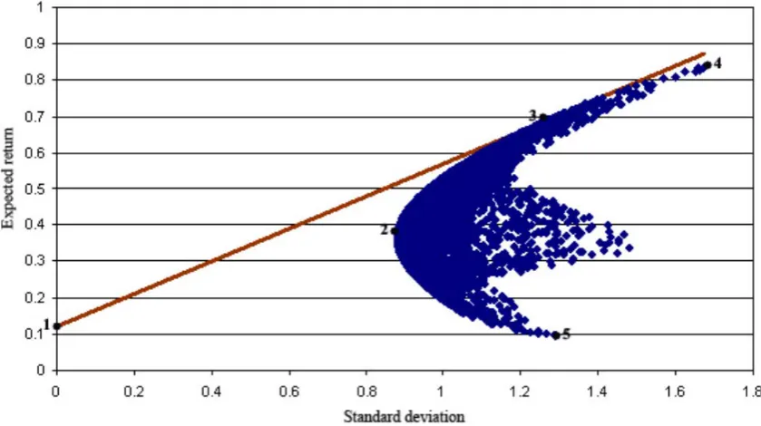
Figure 3.1. The efficient mean-variance portfolio ... 39

Figure 3.2. Time variations in realized equity premium (annual, 1871-2009) ... 58

Figure 3.3. Time variations in realized equity premium (1871-2009, 10-year moving average) ... 58

Figure 3.4. Moving average volatility of the S&P 500 index from January 1990 to January 2010 ... 63

Figure 3.5. News impact curve of the GARCH and the TGARCH models ... 67

Figure 4.1. Median of the credit spread series ... 94

Figure 4.2. Median of the equity volatility series ... 95

Figure 4.3. Median of the distance to default series ... 95

Figure 6.1. Sensitivity of the values of equity and debt to changes in the value of the firm’s assets ... 151

Figure 6.2. Sensitivity of the values of equity and debt to changes in the volatility of firm’s assets ... 152

(15)

CHAPTER 1

INTRODUCTION

1.1. Introduction

This thesis investigates three aspects of the relationship between equity and credit

risks. First, it examines the importance of idiosyncratic and systematic equity risks in

determining the credit spread on corporate bonds. The existing literature focuses on

the relationship between the credit spread and the volatility of equity returns in excess

of market return, hence ignoring the differences of firms’ exposure to systematic risks.

This study fills this gap in the literature by decomposing the equity volatility into

systematic and idiosyncratic components and assessing their relationship with the

credit spread.

Second, the thesis investigates how equity and credit risks impact upon the correlation

between equity and bond returns. The existing studies investigate the unconditional

relationship between the credit spread or the bond yield and the variables deriving from

the structural model of Merton (1974). This study estimates the conditional correlation

between equity and bond returns, and then examines the determinants of this

correlation. This approach enables a more thorough analysis which extends the existing

empirical evidence on determinants of the correlation between equity and bond

returns.

Finally, the thesis examines whether the credit sensitive information contained within

financial accounting data is fully reflected in equity prices. A limited number of existing

studies that focus on the relevance of accounting data in credit markets examine the

incremental information value of financial accounting data in explaining bankruptcies,

credit ratings or the credit default swap premiums. This study extends the existing

literature by considering the relevance of accounting data in explaining variations in the

(16)

The empirical analysis is conducted on a large US data sample covering more than 15

years and consisting of over 350 firms and 700,000 daily observations. The remainder

of this chapter briefly explains the background, contributions, structure of the thesis,

research methodology and main research questions.

1.2. Background and Rationale

Equity instruments (shares) are exposed to market or systematic risk, which is inherent

in the entire market, as well as the specific risks associated with particular shares.

However, finance theory implies that investors should only be compensated for bearing

market risk. Specific risks are diversifiable and therefore exposure to these risks should

not be rewarded.

Debt instruments are exposed to credit risk or the probability that the debt will not be

repaid. They enjoy a higher repayment priority when compared with equity. However,

this reduced risk is accompanied by limited upside potential in the value of such

instruments as debt investors are generally entitled only to receive the principal

amount and the stream of promised interest payments.

Whilst there are significant differences between equity and debt instruments, their

value depends on the same underlying assets of the firm and therefore their risk-return

relationship should be systematically related. The theoretical relationship between

market and credit risk is fully defined by Merton (1974) in his groundbreaking structural

approach, based on the option pricing theory of Black and Scholes (1973), which treats

a firm’s equity capital as a derivative instrument written on its assets.

Acknowledging the limited liability of equity holders, equity can be considered as a call

option on a firm’s assets with the value of debt as the strike price. The difference

between the value of a firm’s assets and debt indicates its credit risk. The economic

incentive of equity holders to hold a firm’s assets decreases as their value falls and

approaches the value of debt, resulting in a higher credit risk. Bankruptcy occurs when

the value of assets drops to the point where it is equal to the value of debt. At this point,

equity holders have no incentive to hold firm’s assets and therefore surrender them to

(17)

The structural model of Merton (1974) provides an analytical solution for the value of

any security depending on the value of firm’s assets as well as the probability of default

and the credit spread in case of debt securities. Furthermore, the structural model fully

describes the relationship between the value of equity and debt securities of the same

firm. Intuitively, an increase in the market value of equity has a positive impact upon

the value of debt since it decreases quasi-market value leverage by definition. The

sensitivity of the value of debt relative to the changes in the value of equity increases

as the leverage or the ratio of debt over equity approaches unity. In other words, the

sensitivity of the value of debt to changes in equity value is highest when the firm is

already in distress.

An increase in the volatility of equity increases the probability that the leverage will

approach unity and trigger default. Therefore, the structural model predicts a negative

correlation between the volatility of equity and the value of debt. However, this

relationship is highly nonlinear. Similar to the marginal change in equity value, the

marginal change in the volatility of equity impacts upon the value of debt more when

the default is more probable.

The structural model is fundamentally based on the assumption that capital markets

are efficient. This assumption has several important implications of which the most

important is that all credit-relevant information is already reflected in equity prices.

Furthermore, the credit and equity markets are perfectly integrated under this

assumption.

The structural model provides a set of empirically testable predictions which have an

academic as well as a practical importance. From an academic perspective, the

structural model is widely utilized and it is one of the most important theoretical finance

models, hence the novel evidence of its empirical performance is an important

contribution to the existing literature. From a practical perspective, a better

understanding of the relationship between equity and debt risk enables an

improvement in the integrated management of these risks which, as Hartmann (2010)

(18)

1.3. Objectives and Contributions of the Thesis

There are a limited number of empirical studies which examine the relationship

between equity and debt securities. Furthermore, the existing studies are in general

based on a limited data samples, spanning short time periods. This thesis is underpinned

by a large sample consisting of over 350 firms and 700,000 daily observations covering

almost 15 years, and including the period of the recent financial crisis which, according

to most recent studies, started in August 2007. The large data sample enables a more

robust regression analysis and examination of empirical results.

The main objectives of this thesis are to examine the following three aspects of the

relationship between equity and debt securities:

1. The relationship between the credit spread on corporate bonds and equity risk. The

existing studies of the relationship between the credit spread and equity volatility

focus on the volatility of equity returns in excess of the market return, implying that

the sensitivity to market movements or beta is equal in cross-section. This study

extends the existing literature by considering the significance of idiosyncratic as well

as systematic equity risks in explaining the variations in the credit spread. The Fama

and French (1993) three factor model is utilized to decompose equity volatility into

its idiosyncratic and systematic components. The credit spread is then regressed on

the equity volatility components in a set of panel data models. Furthermore, the

structural model explicitly controls for the level of credit risk and empirically

examines the interaction between the level of credit risk and equity volatility.

2. The correlation between equity and corporate bond returns . While the existing

studies generally focus on the unconditional correlation, this thesis uses a bivariate

Generalized Autoregressive Conditional Heteroscedasticity (GARCH) model to

estimate the conditional correlation between equity and bond returns, and then

examines how equity volatility and credit risk affect the correlation in a set of panel

data models. This approach enables a deeper regression analysis as well as an

(19)

3. The relevance of accounting data in the measurement of the credit spread . This part

of the thesis investigates whether financial accounting variables contain any credit

sensitive information not yet reflected in equity market based measures of credit

risk. The incremental information value of such accounting variables is assessed by

considering their significance in explaining the variations in the credit spread in

conjunction with the distance to default, and the latter, according to the structural

model, is a sufficient measure of credit risk. A limited number of existing studies

examine the incremental information content of financial accounting data in

explaining bankruptcies, credit ratings and, more recently, the credit default swap

spreads. This study makes an important contribution by documenting the

incremental information content of the spread of corporate bonds in explaining the

credit.

1.4. Structure of the Thesis

The thesis is divided into ten chapters. Following this introductory chapter, Chapter 2

examines the structural approach to credit risk modelling. After briefly presenting the

seminal model of Merton (1974), the chapter discusses the limitations, estimation and

extensions of the structural model in the extant literature.

Chapter 3 reviews the seminal approaches to the valuation of equity. After reviewing

each equity value model, the chapter examines the determinant of equity premium, the

time variations within it, and the estimation of the equity premium.

The study of the relationship between the credit spread and systematic and

idiosyncratic equity risks is presented in Chapters 4 and 5. Chapter 4 reviews the existing

literature, develops hypotheses, and presents the methodology of this thesis, along

with the data sample. The empirical analysis is conducted by regressing the credit

spread on equity volatility, the distance to default of Merton (1974) and a set of control

variables. The regression results are presented in Chapter 5.

The study of the correlation between equity and bond returns is presented in Chapters

(20)

correlation between equity and bond returns, and results of regressing the correlation

on equity volatility, the distance to default and common risk factors.

The study of the relevance of the financial accounting data in the measurement of credit

spread is presented in Chapters 8 and 9. The literature review, hypotheses and research

methodology is presented in Chapter 8. The significance of the market based indicators

(i.e. the distance to default and equity volatility) and financial accounting variables in

explaining variations in the credit spread is considered separately and jointly. The

empirical finding are presented in Chapter 9.

Finally, Chapter 10 summarises the salient findings from the three empirical studies,

discusses their theoretical and practical implications, and draws conclusions. The thesis

ends with a discussion of the main limitations of the thesis and suggestions for further

research.

1.5. Methodological Considerations

1.5.1. Equity Risk

A decomposition of equity returns into systematic and idiosyncratic components is

required in order to examine the relationship between the corporate credit spread and

the changes in the systematic and idiosyncratic equity risks. One approach to the

decomposition (e.g. Campbell and Taksler, 2003; Cremers et al. 2008) is to assume that

all firms’ loadings on systematic risks are equal, and therefore consider equity returns

in excess of a major equity index to be idiosyncratic returns. Since the assumption that

all firms have equal exposure to systematic risks is unrealistic, this thesis uses a bivariate

GARCH model to estimate the correlation between the firm-level equity returns and

systematic risk factors. The systematic equity returns are considered to be the expected

returns implied by the Capital Asset Pricing Model (Sharpe, 1964; Lintner, 1965; Mossin,

1966) and the three factor model of Fama and French (1993). The idiosyncratic returns

are considered to be the difference between the observed returns and the expected

(21)

Equity risk is measured as the volatility of equity returns, commonly estimated as the

standard deviation of equity returns over an arbitrary number of preceding days. The

GARCH modelling is an alternative approach to the estimation of equity volatility. A

GARCH model treats the current equity volatility as a function of innovations in the

equity returns and the past volatility. Unlike the standard deviation, GARCH models fully

captures the time-series behaviour of equity volatility. Therefore, throughout this

thesis, the equity volatility is estimated by GARCH models.

1.5.2. Credit Risk

The structural approach of Merton (1974) is the most important theoretical approach

to credit risk modelling. The structural model expresses credit risk as the difference

between the market value of firm’s assets and the book value of firm’s debt relative to

the volatility of firm’s assets. The basic structural model has been extended by a number

of authors to account for stochastic interest rates, a mean-reverting leverage ratio and

other features. The extended structural models are much more complex to estimate

and there is no evidence that any of them fully address the empirical weaknesses of the

basic structural model. This thesis therefore utilizes the basic structural model to

estimate credit risk.

1.5.3. Regression Analysis

The data set consists of matched equity, bond and accounting variables for n different

firms over t consecutive time periods. This two-dimensional feature of the dataset

implies that the econometric analysis should be undertaken within the panel analysis

framework. A basic panel date model assumes that the data is homogeneous in

cross-section and therefore estimates a single equation for the entire dataset.

This basic panel model, referred to as the constant coefficient model, can be extended

to account for differences in behaviour across firms and through time. A cross-sectional

fixed effects panel model allows the intercept to vary across firms and captures the

unobserved factors which are firm-specific but constant over time. Similarly, a period

fixed effects panel model captures the unobserved factors which are time-specific but

(22)

time-specific unobserved factors. The empirical phenomena this thesis focuses on are

examined in a full set of panel date models.

The research methodology is fully described in chapters 4, 6 and 8.

1.6. Main Research Questions

The specific hypotheses are outlined in each of the methodological chapters (chapters

4, 6 and 8). The main research questions can be outlined as follows:

1. How do the changes in systematic and idiosyncratic equity volatility affect the

credit spread on corporate bonds?

2. How do the changes in equity volatility and credit risk affect the relationship

between equity and bond returns?

3. Do financial accounting data have any incremental information value in

explaining changes in the credit spread, when considered in conjunction with

equity volatility and the distance to default of Merton (1974)?

Answering these three research questions is the task of Chapters 5, 7 and 9 respectively.

Each of these chapters is preceded by a methodology chapter. However, for

completeness, major issues relating to the measurement of the credit and equity risks

are reviewed first. These are dealt with in Chapters 2 and 3 respectively. The next

(23)

CHAPTER 2

THE THEORETICAL FRAMEWORK FOR CREDIT RISK MEASUREMENT

2.1. Introduction

The measurement of credit risk has been one of the most important topics in finance.

The earliest studies used accounting variables to assess the credit risk and classify firms

into different credit groups. In one of the first studies, Beaver (1966) found that key

leverage and cash flow ratios of non-defaulted firms differed significantly from the

ratios of defaulted firms. He also found that these ratios were highly significant in

predicting a firm’s failure to service its contractual obligations. Beaver’s study inspired

a number of researchers to greatly improve performance of accounting-based models

by using better statistical methodology and variables that serve as better proxies for

credit risk.

Accounting-based and other models do not, however, take into account the fact that

markets continuously assess credit risk. Market prices of shares and bonds continuously

change as new information arrives. A change in a firm’s outlook will immediately reflect

on its share and bond prices. Therefore, all information about credit as well as equity

risk is contained in market prices of securities.

This shortcoming is addressed by Merton (1974) who builds on the option pricing theory

of Black and Scholes (1973) to develop the original framework for the structural

approach to the valuation of credit risk.

The structural model treats debt and equity securities as derivatives written on a firm’s

assets, so it presents a unique framework for the analysis of interaction between credit

and equity risk. The objective of this chapter is to review the basic structural model,

(24)

2.2. The Structural Approach

The debt of a firm can be considered as a contingent claim on firm’s assets. Taking into

account limited responsibility of equity holders, they will have an economic incentive

to keep control of the firm’s assets only if their market value exceeds the value of debt.

If the opposite is true, equity holders will turn the firm’s assets to the creditors.

Therefore, equity holders can be viewed as holders of a call option written on firm’s

assets with exercise price equal to the value of debt implying that the firm would go

bankrupt when the market value of its assets reaches the level of debt. The value of

equity at maturity of debt can be expressed as:

m ax(0, )

E = A-D _(2.1)

where

A is the value of firms’ assets

D is the book value of firm’s debt

Following the same logic, the creditors have an obligation to purchase firm’s assets at

the price that equals the value of debt. Their position, therefore, is similar to the short

position in a put option. The value of debt at maturity can be expressed as:

m in ( , )

D = D A _(2.2)

This resemblance of firm’s equity and debt to the call and put options enables the use

of the option pricing methodology to estimate the default probability and therefore to

value the debt. Under the efficient market hypothesis, the market prices of securities

reflect all available information and therefore this approach gives the best possible

estimate of credit risk.

Merton’s (1974) model is derived based on the following assumptions:

1. capital markets are perfect, i.e.

a. assets are divisible, there are no taxes or transaction costs

b. there are sufficient number on investors with comparable wealth levels

so that each investor believes that as many assets as wanted can be

(25)

c. there is a market for borrowing and lending at the same rate of interest

d. short-sale of all assets, with full use of the proceeds, is allowed

2. assets are traded continuously in time

3. the theorem of Modigliani and Miller (1958) that firm’s capital structure is

irrelevant to its value holds

4. the interest rate term-structure is flat and known with certainty and

5. the value of assets follows the following diffusion stochastic process:

( - )

t t t t

dA

=

a d

Adt

+

s

AdX

(2.3)

where

α is the instantaneous expected rate of return on firm’s assets δ is the payout rate to equity and debt holders

σ is the instantaneous volatility of the return on firm’s assets and dX is the standard Wiener process / Brownian motion

Under the above assumptions, Black and Scholes (1973), and Merton (1974) show that

the value of any claim f contingent on the value of firm’s assets A and time t must satisfy

the following parabolic differential equation (Black and Scholes, 1973; Merton, 1974):

2 2 2

2

1

0

2

A

f

A

rA

rf

t

s

A

¶

+

×

¶

+

¶

- =

¶

(2.4)

Solving the above equation with the boundary conditions stated in Equation (2.1), i.e.

the value of equity at the maturity of debt equals the difference between the asset

value and debt or zero if firm’s assets are worth less than the debt value, Black and

Scholes (1973), and Merton (1974) show that the value of equity is as follows:

1 2

( )

rT

( )

t t t

E

=

A N d

-

De

-

N d

(2.5)

where:

A is the value of firm’s assets

D is the book value of firm’s liabilities

T is the time to maturity of debt

(26)

2 1 1 ln( ) 2 t A t A A r T D d T s s æ ö

+_ç + _÷

è ø

=

2 1 A

d

= -

d

s

T

σ is the annualized volatility of returns on firm’s assets.

Acknowledging the fact that the asset value is the sum of the values of debt and equity,

the value of debt is given by:

t t t

D

= -

A E

(2.6)

Alternatively, as shown by Black and Scholes (1973), and Merton (1974), the market

value of debt can be obtained by solving Equation (2.4) with the boundary condition

given in Equation (2.2):

,

( )

2

(

1

)

rT

t MP t t

D

=

D e

-

N d

+

A N

-

d

(2.7)

where all variables are as defined in Equation (2.5). The market value of debt is the

principal value discounted at the risk-free rate increased by the compensation for the

credit risk (i.e. the credit spread):

( ) ,

t t

r c T t MP t

D

=

De

- + (2.8)

Using (2.7) and (2.8), the credit spread is given by:

2 1

1

ln ( ) t ( )

t rT

t

A

c N d N d

T D e

-é ù

= - _ê + - _ú

ë û (2.9)

In his seminal paper, Merton (1974) notes that the assumption of perfect capital

markets can be substantially weakened and the purpose of the interest rate assumption

is to clearly distinguish credit risk form interest rate risk. The Modigliani-Miller theorem

is not necessary, as it is actually proved to be a part of the formal derivation of the

structural model. The assumption of the assets valuation process is crucial. It requires

assets returns to be serially independent in accordance with the efficient market

(27)

The main concept underpinning the structural model is intuitively depicted on the

[image:27.595.126.499.135.382.2]

following illustration.

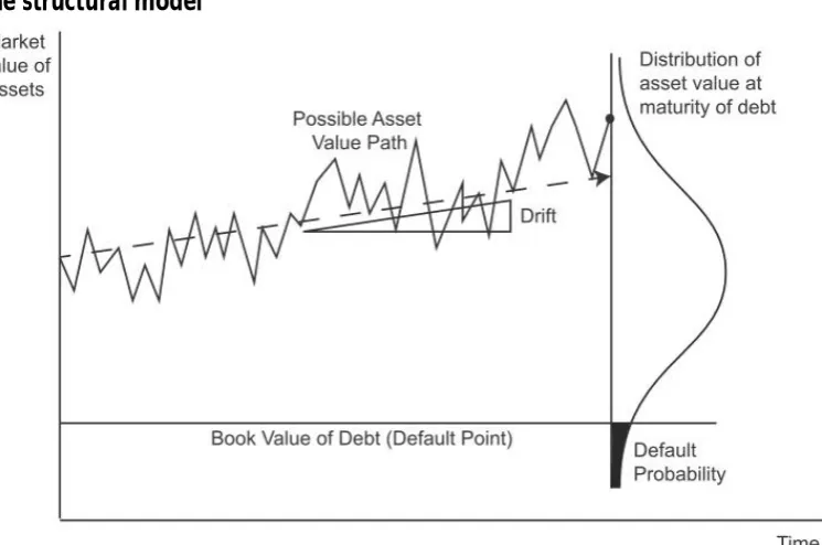
Figure 2.1

The structural model

The distance between the current market value of assets and the book value of liabilities

illustrates the initial leverage. The book value of liabilities is referred to as the default

point because, it is assumed that the firm defaults when the assets value drops to the

book value of liabilities. At that point, the claim the equity holders have on firm’s assets

becomes worthless, so they turn firm’s assets to creditors. As the above figure clearly

illustrates, the analysis of credit risk in the structural model is essentially the evaluation

of the firm’s value, which is assumed to follow the diffusion stochastic process. The

normal distribution of the assets value at the horizon follows from the assumption that

the value of the assets evolves according to the diffusion stochastic process given in

Equation (2.3). The expected rate of return on firm’s assets drifts the value of assets

upward, and thus decreases the probability of default. The volatility of the assets value

is, besides the leverage, the most important parameter. An increase in volatility of the

assets would increase the probability that the assets value would end up below the

book value of liabilities at the horizon triggering default. It should be noted that the

structural model takes into account only assets insolvency, while firms usually fail to

(28)

Another notable approach to the measurement of the credit risk is the reduced-form

approach which, instead of modelling the process of assets value, uses debt securities

directly to estimate the default probability. Classic works in this field include Jarrow,

Lando and Turnbull (1997), and Duffie and Singleton (1999). Unlike the structural

model, reduced-form models do not have a firm structural form. This ensures

tractability and good empirical fit of reduced forms models. On the other hand, the

possibility to choose a functional form of the model necessarily introduces subjectivity.

This may lead to empirical results that exhibit strong in-sample fitting properties but

are inappropriate for drawing conclusions about the population properties. Finally,

reduced-form models do not directly link the values of firm’s debt and equity. They,

therefore, do not provide a comprehensive and theoretically appealing framework for

the analysis of interaction between equity and credit risks.

2.3. Limitations of the Structural Approach

As Anderson and Sundaresan (2000) note, the structural model is attractive on

theoretical grounds because it links the valuation of different financial claims on firms’

assets with economic fundamentals. Since all claims derive their value from the same

assets they are systematically correlated. It is possible, therefore, to use values of one

class of securities to estimate the value of another. By theoretically explaining the

relationships between claims on firm’s assets, the structural model provides a

framework for analysis of the relationship and interaction between different financial

instruments and markets.

Despite its great appeal, the empirical evidence in support of the structural model has

been mixed at best. Researchers generally report that the structural model generates

much lower credit spreads than those observed. The inability of the structural model to

generate realistic credit spreads can be attributed to simplifying assumptions used to

derive the model, difficulties in estimation of parameters required for the

implementation as well as more profound reasons that question the rationale of using

the diffusion stochastic equitation given in Equation (2.3) as a model for the assets

(29)

The most important drawback stems from the assumption that the assets value evolves

continuously as described by Equation (2.3). As illustrated above, the default probability

and therefore the credit spread is implied by the volatility of assets value and the

difference between the asset value and the debt value. This difference divided by

volatility is usually referred to as the distance to default. Due to the fact that

continuously evolving value of assets needs time to change significantly, the default

probability in short time is close to zero. The structural model therefore does not take

into account the risk of large changes in values of assets. This is probably one of the

main reasons why the structural model generates a lower credit spread than those

observed.

Another drawback of the structural model is that the default can only occur at the

maturity of debt and the default is assumed only when the total assets value reaches

the debt value. In addition to this cause of bankruptcy, dubbed as the assets insolvency,

the firm can default because of cash-flow insolvency. Ignoring cash-flow insolvency is

probably another significant reason for the prediction of systematically lower credit

spreads than those observed in the market.

Another obvious drawback is that the structural model is derived under the assumption

that the interest rate term structure is flat and known with certainty. Besides being

unrealistic, this assumption rules out the correlation between the interest rate and the

value of the firm. This correlation is potentially important as the cross-sectional

differences in the sensitivity of firms’ values to the change in the interest rate may exist.

Sweeney and Warga (1986), for example, provide evidence that the changes in the

risk-free rate affect equity returns and that this effect is much stronger for the utility

companies than for the whole market.

2.4. Estimation of the Structural Model

2.4.1. Estimating Unobservable Value of Firm’s Assets and the Volatility of

Assets

Empirical implementation of the structural model is not straightforward. The capital

(30)

used to derive the structural model. Firms usually have different forms of equity (e.g.

common shares, preferential shares, restricted shares etc.) and debt (bank term debt,

short-term debt, straight bonds, convertible bonds etc.) in their capital structures. Due

to the fact that not all components of the firm capital are traded, the market value of a

firm’s assets cannot be directly observed. The empirical research is usually based on

public firms with actively traded shares, so this problem is scaled down to the

estimation of the market value of debt. A closely related issue is the estimation of assets

volatility, which is also not directly observable. Campbell and Taksler (2003), for

example, take the book value of debt as a proxy for its market value and assume two

extreme scenarios for the volatility of debt. In the first scenario, the volatility of debt is

assumed to be zero and in the second, it is considered to be equal to the volatility of

equity. They note that these extreme scenarios are not realistic and call for further

research.

A more sophisticated approach to estimating the assets value and volatility is to take

advantage of the derivative nature of equity and use the option pricing theory to obtain

two equations with two unknown variables (assets value and volatility). The first

equation is the call option pricing formula given in Equation (2.5), i.e.:

1 2

( )

rT

( )

E A N d

=

-

De N d

-where

E is the value of equity

A is the asset value

D is the debt value

σ2_{is the annualized standard deviation of asset returns}

r is the risk-free interest rate

N is the cumulative density of the standard normal distribution

T is the time to maturity of debt

Assuming that the firm’s equity value follows the same stochastic diffusion process as

the asset value, its dynamics under the risk-neutral probability measure can be

(31)

t t E t t

dE rE dt

=

+

s

EdX

(2.10)

where:

r is the risk-free interest rate

σ

E is the annualized standard deviation of returns on the equity

dX is the standard Wiener process

The equity is a function of time and the asset value, i.e.

E

t

=

f V t

( , )

t . Therefore, Itô’s

Lemma can be applied to get:

2

2 2

( , ) ( , ) 1 ( , ) ( , )

( )

2 ( )

t t t t

t t t A t A t

t t t

f A t f A t f A t f A t

dE A r A dt A dX

t A A A

d d _s d _s

d d d

é ¶ ù

=_ê + + _ú +

¶

ë û

(2.11)

The comparison of the coefficient multiplying the Brownian processes in the two

preceding equation gives the following identity:

( , )

_t

E t t A

t

f A t

E

A

d

s

d

=

_(2.12)

Equations (2.5) and (2.12) form a system of two equations with two unknown variables

(the asset value and its volatility). Therefore, it is possible to solve these two equations

simultaneously and obtain estimates for the asset value and the asset volatility. This

appears to be most frequently used method for estimation of unobservable assets value

and volatility. It is advocated by major text books (e.g. Hull 2006, Saunders 1999), and

widely used in academic studies (e.g. Ronn and Verma (1986), Hillegeist et al. (2004),

Das and Hanouna (2009), Cooper and Davydenko (2003), Delianedis and Geske (2003),

and Campbell, Hilscher and Szilagyi (2007)).

Another approach is to adopt an iterative procedure. In this approach, the volatility of

equity, which can be estimated from historical daily prices of equity, is initially

considered as the volatility of assets. This makes it straightforward to estimate the value

of assets, which remain the only unknown variable in the equation. The standard

deviation of the estimated values of assets serves as the volatility of assets in the next

(32)

(2003), and Duffie, Saita and Wang (2007). Also, this approach is used in a commercial

implementation of the structural model by Moody’s KMV (Crosbie and Bohn, 2003).

In support of the iterative approach, Crosbie and Bohn (2003) of Moody’s KMV note

that the estimates obtained by the system of equations method hold only

instantaneously. This implies that these estimates would be acceptable if the leverage

of firms was constant. However, they note that the leverage of firms is not constant,

but experience significant changes. Industrial firms usually increase their leverage as

they approach default, whereas the leverage of financial firms behaves exactly the

opposite. Therefore, they conclude that the system of equations method is unlikely to

yield reasonable results. Bharath and Shumway (2008) provide results that are

inconsistent with this claim. They find that the computationally intensive iterative

approach does not improve model performance.

Duan (1994) proposes a third approach. He points to drawbacks of estimating assets

value and volatility by simultaneously solving two equations as presented above, and

proposes using the maximum likelihood method instead. He argues that the former

method considers assets volatility as constant and independent of assets value and

time. Also, in his view, the two equations that are simultaneously solved are essentially

the same equation which makes one of them redundant. Finally, the two equations

method does not provide confidence intervals for estimated values of assets and

volatility.

Duan (1994) considers observed time series of equity prices as a sample of transformed

data with the call option pricing equation defining the transformation. The maximum

likelihood method is used to find values of assets and volatility which maximises the

likelihood of obtaining equity prices in the sample. Interestingly, Duan notes that his

method provides identical estimates of as those yielded by the iteration method

employed.

Wong and Li (2004) emphasize the importance of the method for estimating market

value of assets and associated volatility. They point that the use of book value of debt

as a proxy for its market value overestimates the value of assets and therefore the

(33)

Ericsson and Reneby (2005) estimate three versions of the structural model and run

simulations to investigate whether the performance of models depend on the method

for estimating assets value and volatility. They find that the maximum likelihood

method clearly dominates the system of equations method and that the latter performs

so poorly that it may be a cause for empirical failures in implementation of the

structural model. In addition to yielding unbiased and relatively efficient parameters,

they point to the maximum likelihood method that allows straightforward derivation of

the probability distribution and thus confidence intervals of parameters.

Suo and Wang (2006) use the maximum likelihood method to estimate the assets value

and volatility using equity as well as bond prices. When bond prices are used, they find

that estimated assets volatility is unreasonably high and that the estimation process

does not converge for most of the observations in their sample.

2.4.2. Choosing Default Point and Time Horizon

The structural model envisages a firm with simple capital structure consisting of equity

and a zero coupon bond. In this setting, the firm defaults if its assets are worth less than

the bond’s face value when the bond matures. As already mentioned, firms’ capital

structures are much more complex. Virtually all balance sheets contain current

liabilities, short-term loans, long-term loans, bonds and other classes of liabilities.

Maturities and other details on firms’ liabilities are not easily accessible. Therefore, a

choice of the default point and the maturity of liabilities is not straightforward, and may

influence empirical results.

As a minimum, the default point should include all liabilities that are due during the

period for which the default probability is modelled. The other extreme is to include

total liabilities, because the firms usually pay interest or coupons on all liabilities. It

should be also taken into account that the ability of firms to refinance their debt

depends on the total leverage.

A review of the literature shows that the most common choice for the default point is

the book value of total liabilities. This choice is adopted by Campbell and Taksler (2003),

(34)

Hillegeist et al. (2004). In its commercial implementation of the structural model,

Moody’s KMV assumes that the default point amounts to the short-term liabilities and

a portion of long-term liabilities (Dwyer and Su, 2007). Following this approach,

Vassalou and Xing (2004) use the short-term debt plus half of the long-term debt and

argue that this choice adequately captures the financing restraints of firms. They

examine the sensitivity of their results to the choice of the proportion of the long-term

debt included in the calculation and find it not large enough to significantly alter their

results. Das and Hanouna (2009) also take into account only fifty per cent of the

long-term debt.

The choice of default point should be related to the choice of the time horizon over

which the default probability is modelled. If the long-term liabilities are included in the

default point then their maturity should play an important role in choosing the time

horizon. Otherwise the model would potentially overestimate the default probability of

firms financed with more long-term liabilities. Although the extension of the structural

model to longer terms is pretty straightforward, the literature review shows that it is

common to estimate a default probability for a period of one year, e.g. Du and Suo

(2003), Hillegeist et al. (2004), Bharath and Shumway (2008).

The relationship between the time horizon and the default probability is highly

nonlinear. It is initially positive and then turns negative as the growth in assets values

outweighs the increase in assets volatility due to the extension of the time horizon.

Therefore, the time extension from the standard one-year model is likely to impact

empirical results. Campbell, Hilscher and Szilagyi (2007) provide a similar empirical

support for this argument. They report that the significance of the distance-to-default

variable in their logit regression depends on the time horizon. Also, the coefficient of

the distance-to-default variable takes the expected negative sign only when the time

horizon is extended for two or three years. Delianedis and Geske (2003) try to

overcome this issue by assuming that a maturity of firms’ short-term and long-term

liabilities is one year and ten years respectively. Huang and Huang (2003) use the

duration of liabilities and Cooper and Davydenko (2003) consider the timeframe as an

endogenous variable and choose the value which makes the modelled credit spread

(35)

2.4.3. Estimating the Expected Growth in the Assets Value

According to the assumed dynamic of the value of assets, described by the stochastic

differential Equation (2.3), the expected growth in the value of assets or drift per unit

of time isα-δ, where α is the instantaneous expected rate of return on firm’s assets and

δ is the payout rate to the equity and debt holders. The expected rate of return on firm’s

assets αcan be considered to consist of two components, the risk-free rate r and the

assets risk premiumξ. This expands the expression for the expected assets growth rate

to r+ξ-δ and brings down the estimation of assets growth rate to the estimation of the

assets risk premium and the assets payout ratio.

A higher assets growth rate implies that the value of assets drifts away from the value

of debt at a faster pace. This causes the distance to default to widen and therefore

lowers the probability of default as clearly depicted in Figure 2.1. Similarly to the assets

value and volatility, the expected asset premium and payout rates are not directly

observable. In his seminal paper, Merton (1974) shows that the value of a derivative

written on a firm’s assets does not depend on the expected growth in the asset value

or the risk preference of investor. In this risk-neutral setting, returns are discounted at

the risk-free rate which makes the estimation of the asset risk premium unnecessary.

This argument provides the theoretical justification for the use of risk-neutral

probability of default.

The literature identifies different approaches to estimation of the asset value growth

rate. Using the risk-neutral probability and therefore avoiding the estimation of the

asset risk premium is the most straightforward approach. The payout rate is computed

as the weighted average of bond's coupon rate and dividend yield where the weights

are derived from the leverage ratio. This approach is utilized by Ericsson et al. (2005),

Huang and Zhou (2008), and Campbell and Taksler (2003).

An alternative approach, used by Vassalou and Xing (2004) and Eom et al. (2004), is to

use the average change in the estimated value of assets as a proxy for the drift

parameter. This approach eliminates the need for estimation of the expected growth

rate and the payout ratio separately, because both rates are reflected in the average

(36)

average change in the estimated asset value, in the iterative procedure discussed in the

previous section. Similarly, Suo and Wang (2006), as well as Ericsson and Reneby (2004)

use the maximum likelihood method to estimate the drift parameter alongside the

assets value and the volatility of assets.

Another notable approach is found in the widely cited paper of Huang and Huang

(2003). They derive the asset risk premium from the equity premium estimated in the

regression analysis by Bhandari (1988). As the payout rate, they take the weighted

average between the average historical dividend yield (four per cent according to

Ibbotson Associates, 2002) and the average historical coupon rate which they estimate

at nine per cent. Applying weights given by the average leverage ratio for S&P 500 index

firms provides them with the payout rate of six per cent. Leland (2004) follows a similar

approach and assumes a payout rate of six per cent and an asset risk premium of four

per cent. Besides computing the payout rate in the usual manner, Ericsson et al. (2005)

consider it to be an exogenous variable taking values of zero or six per cent. Finally, a

proxy for the rate of return on firm’s assets may be an accounting variable. Patel and

Pereira (2005) use the ratio of earnings before interest and taxes to total assets as a

proxy for the expected rate of return on firm’s assets and they follow Huang and Huang

(2003) in assuming the six per cent payout rate.

2.5. Extensions of the Structural Model

Merton’s (1974) seminal paper inspired further research on credit risk modelling based

on the asset valuation process. As a result, a number of extensions of the original

structural model have been proposed. Major works aimed to improve the model’s

performance by relaxing the model’s assumptions and a better modelling of the asset

valuation process. Although the mathematical derivation of these models is to a great

extent more complex than that of the origin

The interaction between equity and credit risks