Improving Accuracy and E
ffi
ciency of Mutual
Information for Multi-modal Retinal Image Registration
using Adaptive Probability Density Estimation
P. A. Legg1,2, P. L. Rosin1, D. Marshall1 and J. E. Morgan3
[email protected], [email protected], [email protected], [email protected]
1School of Computer Science, Cardi↵University, UK. 2Department of Computer Science, University of Oxford, UK. 3School of Vision Sciences and Optometry, Cardi↵University, UK.
Abstract
Keywords: Mutual information; image registration; probability estimation; histogramming.
1. Introduction
Image registration is the task of finding the spatial transformation that gives correct matching correspondence between two images. Registration is widely used in many application areas. In particular, registration of images from di↵erent modalities has become increasingly common in areas such as Medical Imaging for in-depth patient analysis. However, the difficulty is that by their very nature, multi-modal image pairs may have no clearly defined relation between corresponding image intensities.
Mutual Information (MI) has become a popular similarity measure for multi-modal registration. The algorithm was simultaneously proposed by both Viola [1] and Collignon [2], and since then has stimulated much inter-est. Derived from Information Theory, MI is based on statistical comparison between the two images being registered. This di↵ers from traditional reg-istration techniques that rely on direct pixel intensity calculation such as Normalized Cross-Correlation. Given the floating image A and the corre-sponding area from the reference image B, MI can be defined as:
M I(A, B) =H(A) +H(B) H(A, B)
where H(A) is the entropy of imageA,H(B) is the entropy of image B and H(A, B) is the joint entropy of both A and B. The transformation that maximizesM I(A, B)should result in the correct registration. Studholme [3] extended this by introducing Normalized MI that is designed to handle partial overlap of the images. This is defined as:
N M I(A, B) = H(A)+H(B)H(A,B) .
Entropy gives a measure of the amount of information that a given signal may contain, and forms the basis of MI. For a signal X consisting of n elements, Shannon’s entropy [4] is defined as:
H(X) =
n
X
i=0
(a) (b)
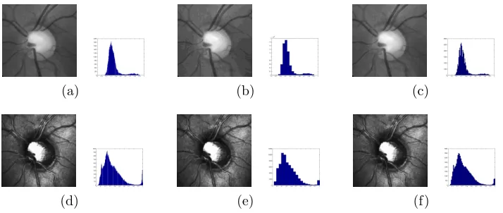
Figure 1: (a) Fundus colour photograph. (b) Scanning laser ophthalmoscope image.
where p(i) is the probability of value i occurring within the data set. The amount of information for a given value is inversely related to its probability, meaning that if the probability of a particular value occurring is low then this returns a greater amount of information than if the probability of the value is high. It can be thought of that the more rare the occurrence of an event, the more important it is when that event does occur. For an image, if there are many identical intensity values (such as background) then the entropy result will be low. However, an image that has lots of detail will return a much larger entropy, due to having a greater variety of intensity values. From this description, entropy can also be thought of as a measure for the dispersion of the probability.
This can be extended further to compute the entropy of two signals, known as the joint entropy. The joint entropy defines the amount of infor-mation given by the combination of both signals. Using Shannon’s entropy, we can define joint entropy of two signals A and B, consisting of n and m elements respectively, as:
H(A, B) =
n
X
i=0 m
X
j=0
p(i, j) log2p(i, j)
where p(i, j) is the probability of value i occurring in A at the same time as j occurs within B. From this, it can be seen that it is the probability distribution of the two images being registered that forms the basis of the MI algorithm. Therefore how the probability distribution is actually estimated could have a significant impact on the performance of the MI algorithm.
[image:3.612.186.425.127.231.2]modalities that are to be registered together are colour fundus photographs and confocal scanning laser ophthalmoscope (SLO) images (Figure 1). Both modalities capture high quality images from the eye of the optic nerve head (ONH), with the fundus photograph recording the clinical appearance and the SLO image providing quantitative information such as the retinal surface reflectivity and topographic structure [5]. Whilst it is apparent that similar features exist in both images it is also very clear that there are significant di↵erences in how these are represented. Fusion of the two images would bring together complementary information and improve ONH analysis for the early detection of glaucoma.
In this paper we conduct a comprehensive study that shows how his-togram bin size estimation methods can heavily impact on MI registration results. We present a number of histogram bin size methods from statis-tics literature (Section 3). We also present alternative probability estimation methods that have also become popular in the literature (Section 4). Using these methods we carry out extensive testing of MI registration (Section 5). Finally, we provide discussion on the study (Section 6).
2. Literature Review
MI relies on a number of factors that need to be carefully considered in order to perform accurate image registration. Pluim [6] gives a thorough survey of the algorithm along with an overview of influencing factors that a↵ect registration performance. Beirlant et al. [7] provides a mathematical overview of entropy estimation methods and discusses the associated param-eters. Paninski [8] also looks at the estimation of entropy methods, and extends this to consider the estimation of MI. The report by Egnal [9] in-troduces the topic of probability estimation in relation to MI well, and also introduces the notion of histogramming in relation to MI.
the number of bins would cover the full range of 256 gray-levels to maintain intensity independence, although not necessarily stated. Collignon et al. [2] do not initially specify bin size, however later work by Maes et al.[11] states that they use 256 bins. They also mention that they do not investigate the influence that bin size may have.
More recent works have began to realise the importance of histogram bin size, however they typically rely on experimental selection rather than on any statistical basis. Dowson and Bowden [12] make the point that MI is not invariant to the bin size, although do not demonstrate the e↵ects of altering this parameter. Lachner states the importance of determining correct bin size based on the trade-o↵ between histogram variance and bias [13], concluding that 64 bins provide satisfactory results for their experiments. In contrast to this, Ritter et al. [14] performs registration of intra-modal fundus pho-tographs using just 4 histogram bins, again determined through experimen-tal testing. Nam et al. [15] experiment using 5, 10 and 32 bins, concluding that 10 bins gives the best results for their data. Similarly, Kang et al. [16] assessed using 4, 8, 16, 32 and 64 bins, concluding that the best number of bins is between 4 and 16. It is often suggested, as in [17], to simply use a power of 2 as a suitable value for bin size, or as in [18], ‘a low number of bins’.
From our review of the literature, it is evident that bin size selection has not been fully explored within MI. However, probability distribution provides the fundamental basis of the algorithm and could dramatically a↵ect the registration performance.
3. Histogram Bin Size Selection
When a continuous analogue signal such as an image is discretized for the purpose of digital processing, artefacts occur due to intensity and spatial quantization. Probability density estimation is the task of predicting the shape of the true distribution based on the sampled data set. By finding the ‘optimal’ probability density representation it may be possible to obtain an estimate close to that of the original signal. Similarly, by adapting the probability density representation further, distracting artefacts such as noise may be reduced to leave only salient features in the image.
The simplest and most common approach to probability density estima-tion is by use of a histogram. Typically, an image histogram shows how many occurrences there are of each independent intensity value within the data set. Each set of occurrences is a ‘bin’ within the histogram. We can also reduce the number of bins to group together intensities. By grouping intensities, we can reduce the number of empty bins that occur within the distribution (since an image will unlikely consist o↵ all possible intensity values). How-ever, reducing the number of bins too far will degrade the information in the image dramatically meaning that distinct features are lost. Histograms tend to take two forms; regular and irregular. When discussing the number of bins for a histogram it is typical to use a regular histogram where bin width is uniform throughout. Irregular histograms, whilst they can provide greater flexibility in classification, would most likely require some intervention by the user which makes this unsuitable for an automated registration procedure.
In Section 2 we have shown that there are many statistical methods for computing bin size selection, although these are not commonly adopted in Computer Vision applications. Unfortunately, of all these methods, there is no single approach that is universally recognized as the best approach for bin size selection. This is because each method relies on assumptions of the underlying data, i.e. what model is chosen to fit that distribution. Typically, how well a model can be fit to the data is measured by a loss function that is to be minimized. The Hellinger Distance and Ln-norms are two common
histogram. For a review of loss functions in application to regular histograms, see Birg´e and Rozenholc [10]. It is the combination of the di↵erent possible distribution models and the di↵erent possible loss functions that leads to the large number of methods in the statistics literature for selecting the possible number of bins.
For our study, we are constructing the histogram for the purpose of further processing, and so we are not concerned with whether the distribution can improve a particular loss function as such. Instead, we assess each method by how well it can improve registration. We wish to minimise the registration error by adopting di↵erent bin size selection methods. The method that results in the least error can be regarded as the most suitable bin size selection method for registration.
3.1. Sturges’ Rule
Sturges’ Rule [20] was originally proposed in 1926 and is still commonly used today in many statistical computer packages. The rule provides a simple formula that is based on properties from the data being classified in the histogram. Sturges’ Rule makes the assumption that a histogram consisting of Normal data can be approximated by a binomial distribution. The rule defines the bin width as w = 1 +log2(n) wheren is the number of elements
within the data set. We can then simply determine the number of bins to be r/w where r is the range of the data set. Since Sturges’ Rule assumes that the data is normally distributed it could then give inaccurate results where this does not hold true.
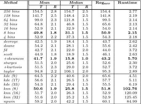
Figure 2 shows an example of applying Sturges’ Rule to the fundus pho-tograph and the SLO image. Both of these images are 259 ⇥266 pixels, meaning that there are 68096 pixels in each image. By applying Sturges’ Rule, it can be seen that the number of bins in the histogram is reduced significantly. For the original fundus image there are 204 occupied bins (i.e. unique intensity values in the image), which can be reduced to just 19 bins after applying Sturges’ Rule. Likewise, for the SLO image this reduction is from 246 to just 19. The number of pixels and the data range are the two main factors in Sturges’ Rule.
(a) (b) (c)
[image:8.612.129.486.123.274.2](d) (e) (f)
Figure 2: Fundus image and associated histogram (a) original, (b) computed using Sturges’ Rule (19 bins), (c) computed using Scott’s Rule (84 bins). SLO image and associated his-togram (d) original, (e) computed using Sturges’ Rule (19 bins), (f) computed using Scott’s Rule (62 bins). Image representations are modified based on the number of histogram bins.
of all probabilities in the data set, which means that if there are less unique intensity values then less calculation is required leading to improved runtime. It is also important to see how the reduced intensity images replicate the originals. It can be seen that the fundus image has lost much detail in the background and created a ‘patch-like’ e↵ect of intensity regions, yet the key features such as the blood vessels and the optic disc still appear very clear. This reduction of intensities could be regarded as ‘cleaning up’ the image, by eliminating noisy artefacts such as the background that could quite easily mislead the registration. In the case of the SLO, whilst there is a similar reduction to the number of unique intensities, the appearance does not look particularly di↵erent. In this situation, the process manages to preserve much of the original detail although we still benefit from the fact that the number of intensities is heavily reduced.
3.2. Scott’s Rule
Scott’s Rule [21] is similar to Sturges’ Rule, however is based on the standard deviation of the data. Given two di↵erent images that have the same intensity range and same size, Sturges’ Rule would give identical bin size whereas Scott’s Rule would give a bin size based on the actual intensity values being considered. Scott’s Rule defines the bin width as 3.49 n 1/3,
within the set. As with Sturges’ Rule, this assumes that the data is Normal. Figure 2 also shows the a↵ect of applying Scott’s Rule to the images. Whereas Sturges’ Rule reduced the number of unique intensity values to just 19, Scott’s Rule suggests that 84 and 62 bins should be used for the fundus photograph and the SLO image respectively. Comparing the histograms, it is clear that Sturges’ Rule reduces the number of intensities greatly and so the histogram now consists of larger steps between each intensity bin. However, Scott’s Rule reduces the bin size whilst maintaining a relatively small step size between each intensity bin in the histogram. For the SLO image, the histogram representation using Scott’s Rule is very similar in shape to that of the original image. This highlights the trade-o↵between using low number of bins whilst trying to preserve the original probability density estimation.
3.3. Variations based on Scott’s Rule and Sturges’ Rule
The introduction of Scott’s Rule gave birth to many variations on the rule that could be used for bin size selection. Taylor [25] and Kanazawa [30] give the bin width as 2.29 2/3n 1/3, whilst Devroye and Gy¨orfi [24] give the bin
width as 2.72 n 1/3. Freedman and Diaconis also took a similar approach
that is described as more robust to Scott’s Rule [31], using the interquartile range (IQR) of the data, which gives the bin width as 2(IQR)n 1/3.
As mentioned previously, both Sturges’ Rule and Scott’s Rule (and its variants) assume that the data consists of a Normal distribution. In Figure 2 it can be seen that this is not the case as both histograms are skewed. Since it is known that the data does not fit the assumptions of the model, the obtained results are likely to be sub-optimal. Typically, it is thought that these methods suggest too few bins (or rather, the equivalent being too large a bin width). Doane [26] proposed a method that extends Sturges’ Rule to account for the skewness of the data. Given thatnis the number of elements, Xi is an element in the set and ¯X is the mean of the set, Doane proposes the
number of bins as:
log2(n) + 1 + log2(1 +
p
b
p
b) where
p
b=
Pn
i=1(Xi X)¯ 3
[Pni=1(Xi X)¯ 2](3/2)
p
b = s
6(n 2) (n+ 1)(n+ 3).
Scott also proposes a method that extends his own method, where Scott’s Rule is multiplied by a skewness factor [27], as defined by:
skewness factor = 2
1/3
e5 2/4
( 2+ 2)1/3(e 2
1)1/2.
By considering the extent of the skew, these approaches tend to recommend using a slightly greater number of bins for the histogram.
Similar to measuring the skewness factor, we can also consider the kur-tosis of a histogram. What the kurkur-tosis measures is how peaked or flat the distribution is in comparison to a Normal distribution. If the data has a high kurtosis then the data has a distinct steep peak close to the mean of the data. A low kurtosis shows that the data has a much flatter distribution. Kurtosis is defined as:
K = Pn
i=1(Xi X)¯ 4
(n 1) 4
where n is the number of elements, ¯X is the mean of the data and is the standard deviation. In Wichard [28], Sturges’ Rule is adapted to include the kurtosis measure, given by:
log2(n) + 1 + log2(1 +K⇤pn/6)
3.4. Joint Histogram Bin Size
In order to compute MI, we need to consider probability estimation from not only the marginal histogram, but also the combined joint histogram. There is little mention in the literature regarding joint histogram bin size selection. Most existing works tend to take the original histogram bins to a power of 2 (e.g. 2562 = 65536 bins). Xie [32] suggests that as a rough
guide, the number of bins used for the joint histogram should give an average of at least one sample per bin. As with the standard histogram, ideally there would be no empty bins within the distribution and so this approach seems plausible, however it is not derived from any statistical justification. Moreover, such an approach is likely to greatly underestimate the number of bins for the joint histogram, resulting in much loss of data with regards to the intensity correspondence between the two images. We decide to use an m⇥ n joint histogram, where m is the number of bins to use for our floating image andn is the number of bins to use for our reference image, as determined by the bin size selection methods discussed previously. In doing this, we maintain the statistical relationship with the marginal probability estimation. This approach eliminates a large number of redundant empty bins compared to when using 2562 bins, whilst also preserving enough bins to
ensure that the probability estimation remains meaningful. We acknowledge that this approach is not optimal, however it does serve to draw the attention of the community to the importance of bin size in joint probability estimation. The topic of joint probability estimation remains a largely unexplored topic for MI, and is outside the scope for this current work.
4. Alternative Methods for Probability Density Estimation
Along with histogram bin size we also investigate into alternative prob-ability estimation methods which we include in our experimental testing. Whilst these methods are more computationally demanding, it is thought that they give a closer representation of the original signal.
4.1. Kernel Density Estimation
reduces the e↵ect of discrete bin entries. The shape of the kernel determines how the data is spread in the distribution. To show how this method relates to the histogram, supposing we chose the kernel to be a square block, with a width equal to our histogram bin width, then this would essentially be equivalent to our original histogram. However, if we choose the kernel to be a smooth Gaussian curve, this can provide a much more desired result. Similar to this is the idea of using a B-Spline curve to spread the probability distribution in the same fashion [34]. As well as the shape of the kernel, we need to ensure that the kernel size is chosen well to suit the distribution. If the kernel is too small or too large this would lead to an under-smoothed or over-smoothed distribution respectively.
4.2. k-Nearest Neighbour Density Estimation
The k-Nearest Neighbour (kNN) approach [35] is a commonly used tool for classification that relies on computing the average distance between a given point and its k-nearest neighbours within the data set. Clearly this method is highly dependent on neighbouring data points, and also takes into account the spread of the data. Essentially, kNN is closely related to KDE then. In KDE, the kernel remains a fixed size and captures a variable number of samples at each data point. In kNN, the kernel size becomes variable so as to capture a fixed number of samples as defined by k. As with previous methods, careful parameter selection for k is important, causing an under-smoothed or over-under-smoothed distribution if set too low or too high. In the current literature, it is recognized that kNN can be very computationally expensive for large data sets [36]. This is due to computing the size of the kernel based on the neighbourhood points for every element in the data set. In the context of MI registration, this could easily become exceptionally expensive leading to an impractical system for performing fast registration.
4.3. NP-Windows
the intensities that occur within the triangle area. Each intensity bin is then incremented based on the area of the two triangles. This approach accounts for absent intensity variations between a pixel and its neighbour, as before, aiming to reduce the artefacts introduces by pixel discretization. Rajwade proposed a similar idea [38] that interpolates the image to an infinite reso-lution. This approach could be seen as histogram interpolation, whereby we could scale the histogram by a given factor and then scale back to the original size. The scale factor would a↵ect how much smoothing is introduced into the histogram, but also lead to expensive computation to perform. Com-pared to standard histogram binning this method is very slow to compute, which due to computational demands of the algorithm is not surprising. We note that the authors’ work suggests using GPU optimization to compute NP-Windows in a satisfactory time, however this is beyond the scope of our study.
5. Evaluation of Probability Density Estimation Methods
impact both the registration accuracy and runtime efficiency. A naive ap-proach would use an exhaustive search that considers all possible transfor-mations. Even for just rigid transforms only (rotation and translation) this is far too time-consuming and not practical. Instead, an optimized search scheme is required. In our testing we shall consider two well-known optimiza-tion methods; Nelder-Mead Simplex and Simulated Annealing (details and implementation for each of these can be found in [40]). Whilst these schemes can speed up the search process, it should be noted that they can also give incorrect results should the search space contain local maxima that ‘trap’ the search process. Therefore it is important that the search scheme works well in conjunction with the similarity measure. We choose Nelder-Mead Simplex and Simulated Annealing since these are two common optimization methods that are well-known within the community. While many alternative search optimization schemes exist, it should be recognized that the main focus of this paper is to improve the similarity measure being optimized. By improv-ing the convergence of the similarity measure, there becomes less uncertainty in the performance of the optimization method.
Another possible technique to improve registration is the inclusion of a multi-resolution image pyramid. Registration is performed at the coarse (top) level of the pyramid which acts as the initialization point for the next level down. This is done for each level of the pyramid until reaching the fine (bottom) level which consists of the original image. This approach can dra-matically improve runtime since the low resolution images can be processed quicker and are used to initialize registration of the high resolution images. Multi-resolution pyramids are also commonly used in 3D and 4D registration schemes. So whilst the original image data may have many more data points than our 2D registration example, the coarse levels of the pyramid will ac-tually be quite similar, meaning that the same bin size strategies could be applied also.
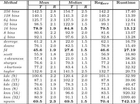
reg-Method Mean Median Regerr Runtime
T R T R
256 bins 154.5 2.8 154.7 2.5 154.4 2.77
128 bins 141.7 2.5 148.4 2.5 141.8 2.19
64 bins 99.0 2.3 121.8 1.5 99.5 2.14
32 bins 64.8 2.1 46.8 1.5 65.6 2.13
16 bins 52.9 2.1 32.9 1.5 54.0 2.14
8 bins 49.8 1.8 31.1 1.5 50.9 2.15
4 bins 52.9 2.2 37.3 1.5 54.3 2.18
devroye 42.5 1.9 18.4 1.5 43.7 2.62
doane 54.2 2.1 28.1 1.5 55.6 2.42
fd 42.7 2.1 22.0 2.0 44.0 3.72
scott 44.9 1.8 18.9 1.5 46.1 2.63
+skewness 41.7 1.9 15.8 1.0 43.2 5.70
sturges 51.5 2.0 25.6 1.5 52.6 2.30
+kurtosis 51.5 2.3 29.0 2.0 52.7 3.72
taylor 94.8 2.2 106.1 2.0 95.3 2.89
kde (9) 64.5 2.2 40.6 2.0 65.6 4.51
kde (17) 56.6 2.1 26.5 1.5 57.7 5.11
kde (33) 54.3 2.1 29.4 1.5 55.5 6.19
knn (8) 50.6 1.9 25.8 1.5 51.8 102.76
knn (16) 51.7 2.0 26.3 1.5 52.9 120.09
knn (32) 51.6 2.0 25.2 1.5 52.9 125.45
[image:15.612.191.420.125.295.2]npwin 59.2 2.0 42.2 1.5 60.1 84.99
Table 1: Registration error results: MI combined with an image pyramid using simplex search. Table shows fixed bin size (top), adaptive bin size (middle), and alternative esti-mation methods (bottom). Translation and Regerr are given in pixels, rotation is given in degrees, and runtime is given in seconds.
istration algorithm, and aims to minimize the possible error that could be introduced by using a search optimization strategy. As the pyramid is tra-versed the rotation search space becomes further restricted, converging to a fixed parameter by the lowest level of the pyramid. For our testing where no image pyramid is used, the full rotation range is allowed throughout the registration.
For our study, we developed a MATLAB implementation for perform-ing multi-modal image registration. For search optimization, we use the built-in MATLAB implementation of the Nelder-Mead simplex algorithm
(fminsearch), and the implementation by Vandekerckhove of Simulated
An-nealing (available from MATLAB Central [41]). Experiments were conducted on a standard desktop PC machine configured with a Pentium 2.6GHz dual-core processor, 4GB of memory, and Windows 7 operating system. The regis-tration software developed and a subset of the image data are both available to download by request to the authors.
5.1. Registration Error Results
Method Mean Median Regerr Runtime
T R T R
256 bins 142.5 2.8 154.7 2.5 142.2 17.40
128 bins 140.1 2.5 141.3 2.0 140.2 13.39
64 bins 125.7 2.3 137.5 2.0 125.9 12.64
32 bins 98.5 2.1 122.9 1.5 99.1 12.71
16 bins 78.9 1.9 84.8 1.5 79.5 13.12
8 bins 80.6 2.2 92.9 2.0 81.6 13.07
4 bins 92.1 2.5 97.6 2.5 92.8 13.28
devroye 61.2 1.8 22.0 1.5 62.1 16.79
doane 76.1 2.0 82.5 1.5 76.9 15.49
fd 45.6 1.9 27.6 1.5 46.6 27.19
scott 55.9 1.8 23.0 1.5 56.9 16.80
+skewness 57.4 1.9 21.0 1.5 58.3 38.26
sturges 76.6 2.1 70.3 1.5 77.2 14.33
+kurtosis 77.2 2.1 83.4 1.5 78.1 32.32
taylor 132.6 2.4 141.5 2.5 132.7 20.73
kde (9) 100.6 2.2 120.4 2.0 101.1 32.99
kde (17) 87.1 2.4 102.2 2.0 87.8 39.06
kde (33) 76.6 1.9 78.3 1.5 77.3 49.47
knn (8) 83.5 1.9 103.3 1.5 84.3 894.54
knn (16) 82.9 2.1 96.6 2.0 83.5 920.32
knn (32) 80.9 2.0 91.1 1.5 81.4 1099.40
[image:16.612.191.421.125.295.2]npwin 69.5 2.3 69.5 1.5 70.4 742.13
Table 2: Registration error results: MI combined with an image pyramid using simulated annealing. Table shows fixed bin size (top), adaptive bin size (middle), and alternative estimation methods (bottom). Translation andRegerrare given in pixels, rotation is given in degrees, and runtime is given in seconds.
registration error based on the 4 corner points of the template image, defined asRegerr (measured in pixels). This is calculated by measuring the distance
for each corner point between the registration result and the ground truth. Each experiment is carried out using the complete set of 135 retinal image pairs. Four scenarios were tested in our experiments: MI with an Image Pyramid, NMI with an Image Pyramid, MI without an Image Pyramid and NMI without an Image Pyramid. In this paper we report only the most significant results. The complete set of results can be found in [42].
5.1.1. MI with a Multi-Resolution Image Pyramid
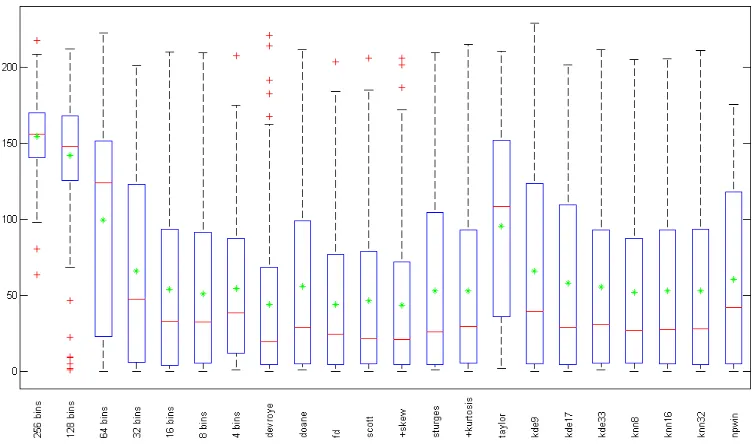
Figure 3: Boxplot of Regerr for MI simplex registration. Bounding box defines the interquartile range, the star defines the mean and the bar across defines the median. Whiskers define the range and the cross defines any outliers.
number of bins through experimental testing. Of the fixed bin methods, it can be seen that 8 bins gives the lowest registration error when using Simplex and 16 bins gives the lowest registration error when using Simulated Annealing. However, in both cases, using fewer bins than this meant that the registration error increased. This shows then that by using too few bins will degrade registration since salient features in the image are being lost.
When using statistical bin size methods the registration error is reduced further. From these results there are four methods that perform consis-tently better than fixed bin methods and the advanced probably estimation methods: Devroye’s, Freedman-Diaconis’, Scott’s and Scott’s Rule with the skewness factor. The only method that seems to perform poorly in relation to the others is that of Taylor and Kanazawa, giving a result similar to using 64 fixed bins. For the four methods that perform best, it can be seen that Scott’s Rule combined with the skewness factor gives the lowest translation error T, whilst Scott’s Rule gives the lowest rotation error R. If we consider only the registration error as given by Regerr, it is Scott’s Rule with the
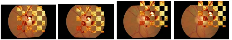
[image:17.612.117.495.123.347.2]reg-Figure 4: MI registration using four di↵erent binning methods. (a) Scott’s Rule, (b) 4 bins, (c) 8 bins, (d) 16 bins. Of all methods, only (a) aligns the images correctly.
istration error. These results clearly suggest that statistical bin size selection helps to improve the result for MI registration. Figure 3 shows this trend using a box plot. The mean registration error Regerr can be plotted for each
method allowing us to visualize the results in a clear and concise manner. Figure 4 shows a registration example using Scott’s histogram rule com-pared to using fixed histogram bin size. In each case where fixed bin size is used, MI fails to successfully register the two images together. The same is also true for when larger fixed bin sizes were used (32, 64, 128 and 256 bins). However, we see that when Scott’s rule is used for adaptive bin size selection, the two images are aligned correctly. This highlights the important fact that careful bin size selectionis required and that it is not simply just a case of se-lecting a low number of bins as has previously been suggested [14, 18, 15, 16].
5.1.2. Overview of remaining testing scenarios
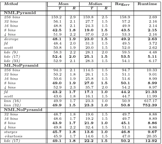
Tables 3 and 4 give an overview of registration error for our remaining testing scenarios: NMI using an image pyramid, MI with no pyramid and NMI with no pyramid. The complete set of results can be found in [42].
[image:18.612.119.495.124.190.2]Method Mean Median Regerr Runtime
T R T R
NMI Pyramid
256 bins 159.2 2.9 159.8 2.5 158.9 2.69
32 bins 56.1 2.1 27.7 1.5 57.2 2.16
16 bins 48.8 2.1 24.3 1.5 49.9 2.14
8 bins 42.5 1.8 19.0 1.5 43.5 2.15
4 bins 51.9 2.2 37.0 2.0 53.3 2.16
devroye 48.1 1.9 23.0 1.5 49.2 2.63
fd 48.4 2.0 31.3 1.5 49.5 3.72
scott 50.8 1.9 20.0 1.5 52.0 2.62
kde (9) 58.3 2.2 28.1 2.0 59.5 4.48
kde (17) 52.4 2.0 25.1 1.5 53.5 5.11
kde (33) 52.9 2.1 28.3 1.5 54.1 6.17
MI NoPyramid
256 bins 94.3 2.1 114.5 1.5 94.7 10.33
32 bins 50.2 1.8 26.1 1.5 51.1 9.01
16 bins 50.6 1.9 25.8 1.5 51.6 8.99
8 bins 49.0 1.9 27.0 1.5 50.1 8.99
4 bins 52.9 2.3 35.7 2.0 54.2 8.97
fd 43.2 1.7 17.1 1.0 44.2 21.33
scott 43.6 1.8 16.1 1.5 44.7 11.99
knn (16) 49.9 1.7 23.3 1.0 50.9 617.17
knn (32) 49.9 1.5 23.3 1.0 50.8 752.39 NMI NoPyramid
32 bins 48.7 1.8 19.6 1.5 49.7 8.88
16 bins 48.6 1.7 19.2 1.5 49.7 8.89
8 bins 43.9 1.7 21.9 1.0 45.1 8.86
4 bins 49.8 2.2 32.4 1.5 51.1 8.86
sturges 45.7 1.8 13.6 1.0 46.8 9.67
+kurtosis 45.9 1.7 14.6 1.5 47.0 20.35
[image:19.612.176.436.123.355.2]kde (17) 49.1 1.8 22.2 1.5 50.2 12.92
Table 3: Registration error results using simplex search for three scenarios: NMI com-bined with an image pyramid, MI with no pyramid, NMI with no pyramid. (Summary of significant results shown). Translation andRegerr are given in pixels, rotation is given in degrees, and runtime is given in seconds.
within the search space. Likewise, it is interesting to observe the di↵erence between when using an image pyramid. It can be seen that registration per-forms best when no image pyramid is used, however runtime is significantly increased. The issue of local maxima becomes more apparent when the im-age pyramid is used, to the extent that in some cases the registration fails to recovers at the lower levels of the pyramid. Whilst the improvement to runtime is beneficial, the accuracy of the registration is vital, and so the similarity measure should aim to reduce the occrrence of local maxima.
ap-Method Mean Median Regerr Runtime
T R T R
NMI Pyramid
256 bins 146.6 2.5 148.4 2.0 146.8 24.11
32 bins 104.6 2.1 127.0 2.0 105.2 14.26
16 bins 78.4 2.1 81.3 1.5 79.1 14.39
8 bins 75.9 2.2 83.5 1.5 77.2 14.37
4 bins 87.6 2.4 91.2 2.0 88.3 14.16
devroye 91.7 2.1 108.2 1.5 92.2 19.53
fd 65.8 1.9 49.3 1.5 66.4 33.65
scott 83.9 2.1 90.7 1.5 84.4 19.61
kde (9) 105.8 2.3 130.4 2.0 106.5 42.46
kde (17) 90.9 2.1 106.2 1.5 91.4 49.59
kde (33) 84.6 2.2 100.1 2.0 85.5 65.20 MI NoPyramid
256 bins 58.3 1.8 47.5 1.5 59.1 70.93
32 bins 35.3 1.7 6.1 1.0 36.5 54.54
16 bins 35.1 1.7 6.3 1.0 36.3 57.39
8 bins 43.2 1.9 18.1 1.5 44.4 57.81
4 bins 52.4 2.1 46.1 1.5 53.4 58.64
fd 28.1 1.6 5.4 1.0 29.1 152.99
scott 26.3 1.5 5.4 1.0 27.5 76.29
knn (16) 27.2 1.5 6.1 1.0 28.9 4983.70
knn (32) 27.5 1.6 6.1 1.0 29.4 5217.90
NMI NoPyramid
32 bins 34.7 1.6 5.7 1.0 35.7 63.84
16 bins 37.2 1.6 6.7 1.0 38.1 60.30
8 bins 40.0 1.6 12.4 1.0 41.1 60.04
4 bins 51.1 2.1 39.7 2.0 52.2 60.11
sturges 35.8 1.6 6.3 1.0 36.8 65.33
+kurtosis 30.6 1.6 5.1 1.0 31.8 175.54
[image:20.612.174.437.124.355.2]kde (17) 37.9 1.9 7.6 1.0 39.0 100.71
Table 4: Registration error results using simulated annealing for three scenarios: NMI combined with an image pyramid, MI with no pyramid, NMI with no pyramid. (Summary of significant results shown). Translation andRegerr are given in pixels, rotation is given in degrees, and runtime is given in seconds.
proach means that it is not suitable for use in a registration scheme. Of course, as we have already discussed, the methods with low runtime may not necessarily provide the correct registration, and so there is a trade-o↵
between runtime and accuracy. Computing MI using Scott’s rule with no pyramid, and searching with simulated annealing we achieve a runtime of 76.29 seconds. This runtime is reasonably acceptable and also delivers the greatest registration accuracy.
6. Discussion
(a) (b) (c)
[image:21.612.144.470.121.372.2](d) (e) (f)
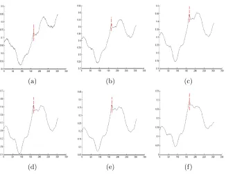
Figure 5: Surface plots showing MI (y-axis) vs. X-Translation (x-axis) using fixed bin sizes. (a) 256, (b) 128, (c) 64, (d) 32 (e) 16 and (f) 8 bins. The red line indicates the point that should be maximized by MI in each plot.
number of fixed bins [17], which we observe in our results can improve reg-istration. We have incorporated adaptive bin size techniques from statistics literature within registration, and found Scott’s Rule, Scott’s Rule with the skewness factor, Devroye’s Rule and Freedman-Diaconis’ Rule, to give the most accurate registration.
MI results when registering a pair of retinal images (Figure 1), computed only for the X-translation, using di↵erent bin sizes. Reducing the parameter space allows us to clearly visualize the di↵erence in the similarity measure. The expected point of registration is given by the dashed vertical line. Using 256 bins, the true registration is a local maximum but not the global maximum. As the bin size is reduced, the true registration becomes more prominent. Even when the true registration is the global maximum (32, 16 or 8 bins), there are other local maxima that could impact on the search strategy. It has been discussed previously that a sparsely-populated histogram will give poor estimation of entropy [43]. By using statistical methods, we can now determine a suitable number of bins rather than simply choosing an arbitrary number of bins in the hope that it performs well.
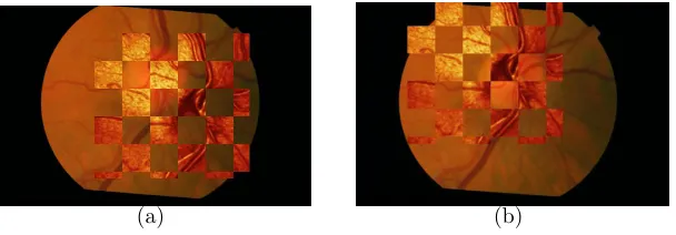
Interestingly, in some particularly challenging cases, we found that the failure of registration to be as a result of weaknesses in the MI algorithm. Figure 6 shows an example of this from our retinal image dataset. In 6(a), MI fails to register the two images. However, the MI score is actually maximized, giving a better result than the ground truth registration 6(b). This result is noticeable for this particular example for all probability estimation meth-ods covered in this study. This highlights that whilst statistical probability estimation may improve upon traditional techniques, MI is still not a fully reliable similarity measure. Kubecka et al. [44] also studied the registration of these two image modalities using MI, and whilst they did not consider the a↵ect of bin size estimation, they did conclude that “the mutual information had global extreme out o↵the point of subjective registration”. They do not give quantitative results for using MI. It is recognized that MI lacks spatial information [6], which if this was incorporated into the algorithm could help to improve registration performance. Some more recent methods consider this (e.g., [45, 46, 47, 48]), however they are more computational-intensive than MI and have significantly longer runtime requirements.
7. Conclusion
con-(a) (b)
Figure 6: An example of difficult registration. (a) Registration given by maximum MI. (b) Ground truth registration.
ducted a comprehensive empirical study for performing image registration that demonstrates the impact of adaptive bin size selection methods, as well as other registration parameters such as search optimization strategies and inclusion of an image pyramid. We show that this approach can improve upon fixed bin size methods, and significantly reduces the need for extensive experimental testing to find a suitable number of bins [14, 13, 15, 16].
Previously, many MI registration applications have focused on common modalities such as MR and CT imaging without much concern regarding bin size, and have enjoyed great success. As more advanced imaging technolo-gies are introduced though, traditional MI registration may not suffice for accurate results. We have seen that this is the case for multi-modal reti-nal images, and that registration parameters needs to be considered more carefully for challenging modalities. Likewise, we would expect that other modalities such as PET/CT registration would also benefit from adaptive bin size selection. More recently, MI has received criticism for not including spatial information, and so new algorithms have been proposed to tackle this. However, MI remains as a simple and reliable similarity measure that can be easily implemented and is fast to compute compared to more modern meth-ods. In addition, the use of adaptive histogram bin size selection methods can yield significant improvements on the traditional MI algorithm, meaning that it should not be neglected for modern registration tasks.
References
[2] A. Collignon, F. Maes, D. Delaere, D. Vandermeulen, P. Suetens, and G. Marchal. Automated multimodality medical image registration using information theory. In Proc. 14th Int. Conf. Information Processing in Medical Imaging; Computational Imaging and Vision 3, pages 263–274, 1995.
[3] C. Studholme, D. L. G. Hill, and D. J. Hawkes. An overlap invariant entropy measure of 3D medical image alignment. Pattern Recognition, 32(1):71–86, 1999.
[4] C. E. Shannon. A mathematical theory of communication. Bell System Technical Journal, 27:379–423, 623–656, 1948.
[5] C. Y. Mardin, F. K. Horn, J. B. Jonas, and W. M. Budde. Preperimetrix glaucoma diagnosis by confocal scanning laser tomography of the optic disc. British Journal of Ophthalmology, 83:299–304, 1999.
[6] J. P. W. Pluim, J. B. Antoine Maintz, and M. A. Viergever. Mutual information based registration of medical images: A survey.IEEE Trans. Med. Imaging, 22(8):986–1004, 2003.
[7] J. Beirlant, E. J. Dudewicz, L. Gy¨orfi, and E. C. Meulen. Nonpara-metric entropy estimation: An overview. International Journal of the Mathematical Statistics Sciences, 6:17–39, 1997.
[8] L. Paninski. Estimation of entropy and mutual information. Neural Computation, 15:1191–1254, 2003.
[9] G. Egnal. Image registration using mutual information. Technical re-port, University of Pennsylvania, 1999.
[10] L. Birg´e and Y. Rozenholc. How many bins should be put in a regular histogram. Technical report, Universit´e Paris VI, UMR CNRS 7599, Universit´e du Maine, 2002.
[11] F. Maes, A. Collignon, D. Vandermeulen, G. Marchal, and P. Suetens. Multimodality image registration by maximization of mutual informa-tion. IEEE Trans. Med. Imaging, 16(2):187–198, 1997.
[13] R. Lachner. From Nano to Space. Springer Berlin Heidelberg, 2008.
[14] N. Ritter, R. A. Owens, J. R. Cooper, R. H. Eikelboom, and P. P. Van Saarloos. Registration of stereo and temporal images of the retina. IEEE Trans. Med. Imaging, 18(5):404–418, 1999.
[15] H. Nam, R. A. Renaut, K. Chen, H.Guo, and G. E. Farin. Improved inter-modality image registration using normalized mutual information with coarse-binned histograms.Communications in Numerical Medthods in Engineering, 25:583–595, 2009.
[16] J. Kang, C. Xiao, M. Deng, J. Yu, and H. Liu. Image registration based on harris corner and mutual information. In Electronic and Mechanical Engineering and Information Technology (EMEIT), 2011 International Conference on, volume 7, pages 3434 –3437, aug. 2011.
[17] Y. Zhu and S. M. Cocho↵. Influence of implementation parameters on registration of MR and SPECT brain images by maximization of mutual information. Journal of Nuclear Medicine, 43(2):160–166, 2002.
[18] J. Tsao. Interpolation artifacts in multimodality image registration based on maximization of mutual information. IEEE Trans. Med. Imag-ing, 22(7):854–864, July 2003.
[19] P. L. Davies, U. Gather, D. Nordman, and H. Weinert. Constructing a regular histogram - a comparison of methods. Technical report, Techni-cal University Eindhoven, 1997.
[20] H. A. Sturges. The choice of a class interval. American Statistical Association, pages 65–66, 1926.
[21] D. W. Scott. On optimal and data-based histograms. Biometrika, 66(3):605–610, 1979.
[22] R. J. Hyndman. The problem with Sturges’ rule for constructing his-tograms. Technical report, Melbourne University, Australia, 1995.
[24] L. Devroye and L. Gy¨orfi. Nonparametric density estimation: The L1
view. Journal of the Royal Statistical Society. Series A (General)., 148(4):392–393, 1985.
[25] C. C. Taylor. Akaike’s information criterion and the histogram.
Biometrika, 74:636–639, 1987.
[26] D. P. Doane. Aesthetic frequency classifications. The American Statis-tician, 30(4):181–183, November 1976.
[27] D. W. Scott. Multivariate density estimation: theory, practice and vi-sualization. John Wiley and Sons, 1992.
[28] J. D. Wichard, R. Kuhne, and A. ter Laak. Binding site detection via mutual information. Proc. of the IEEE World Congress on Computa-tional Intelligence, pages 1770–1776, June 2008.
[29] Hideaki Shimazaki and Shigeru Shinomoto. A method for selecting the bin size of a time histogram. Neural Comput., 19(6):1503–1527, June 2007.
[30] Y. Kanazawa. Hellinger distance and akaike’s information criterion for the histogram. Statistics & Probability Letters, 17:293–298, 1993.
[31] A. J. Izenman. Recent developments in nonparametric density estima-tion. Journal of the American Statistical Association, 86(413):205–224, 1991.
[32] H. Xie, L. E. Pierce, and F.T. Ulaby. Mutual information based reg-istration of SAR images. Geoscience and Remote Sensing Symposium, IGARSS ’03. Proc. IEEE International, 6:4028–4031, July 2003.
[33] N. Kwak and C. Choi. Input feature selection by mutual information based on Parzen Window. IEEE Transactions on Pattern Analysis and Machine Intelligence, 24(12):1667–1671, 2002.
[34] C. O. Daub, R. Steuer, J. Selbig, and S. Kloska. Estimating mutual information using b-spline functions - an improved similarity measure for analysing gene expression data. BMC Bioinformatics, 5:118, 2004.
[36] N. Nicolaou and S. J. Nasuto. Mutual information for EEG analysis.
Proc. 4th IEEE EMBSS UKRI Postgraduate Conference on Biomedical Engineering and Medical Physics (PGBIOMED’05), pages 23–24, 2005.
[37] N. D. H. Dowson, R. Bowden, and T. Kadir. Image template matching using mutual information and NP-windows. In ICPR (2), pages 1186– 1191, 2006.
[38] A. Rajwade, A. Banerjee, and A. Rangarajan. Continuous image repre-sentations avoid the histogram binning problem in mutual information based image registration. In ISBI, pages 840–843, 2006.
[39] Heidelberg Engineering, Heidelberg, Germany. Quantitative Three-dimensional Imaging of the Posterior Segment with the Heidelberg Retina Tomograph, 1999.
[40] W. K. Pratt. Digital Image Processing. Wiley, New York, 2 edition, 1991.
[41] J. Vandekerckhove. General simulated annealing algorithm
(http://www.mathworks.com/matlabcentral/fileexchange/10548),
MATLAB central file exchange, June 2008.
[42] P. A. Legg. Multimodal retinal imaging: Improving accuracy and ef-ficiency of image registration using Mutual Information. PhD thesis, School of Computer Science and Informatics, Cardi↵ University, 2010.
[43] L. Paninski. Estimating entropy onm bins given fewer thanm samples.
IEEE Trans. on Information Theory, 50(9):2200–2203, September 2004.
[44] L. Kubecka, M. Skokan, and J. Jan. Registration of bimodal retinal images - improving modifications. Engineering in Medicine and Biology Society, 2003. IEMBS ’03. 25th Annual International Conference of the IEEE, 1:599–602, September 2003.
[45] P. A. Legg, P. L. Rosin, D. Marshall, and J. E. Morgan. A robust solu-tion to multi-modal image registrasolu-tion by combining mutual informasolu-tion with multi-scale derivatives. InMICCAI, volume 1, pages 616–623, 2009.
[47] D. Rueckert, M. J. Clarkson, D. L. G. Hill, and D. J. Hawkes. Non-rigid registration using higher-order mutual information. Medical Imaging: Image Processing, pages 438–447, 2000.