Besting the Quiz Master:
Crowdsourcing Incremental Classification Games
Jordan Boyd-Graber iSchool and UMIACS University of Maryland
Brianna Satinoff, He He, and Hal Daum´e III Department of Computer Science
University of Maryland
{bsonrisa, hhe, hal}@cs.umd.edu
Abstract
Cost-sensitive classification, where thefeatures used in machine learning tasks have a cost, has been explored as a means of balancing knowl-edge against the expense of incrementally ob-taining new features. We introduce a setting where humans engage in classification with incrementally revealed features: the collegiate trivia circuit. By providing the community with a web-based system to practice, we collected tens of thousands of implicit word-by-word ratings of how useful features are for eliciting correct answers. Observing humans’ classifi-cation process, we improve the performance of a state-of-the art classifier. We also use the dataset to evaluate a system to compete in the incremental classification task through a reduc-tion of reinforcement learning to classificareduc-tion. Our system learnswhento answer a question, performing better than baselines and most hu-man players.
1 Introduction
A typical machine learning task takes as input a set of features and learns a mapping from features to a label. In such a setting, the objective is to minimize the error of the mapping from features to labels. We call this traditional setting, where all of the features are consumed,rapaciousmachine learning.1
This not how humans approach the same task. They do not exhaustively consider every feature. Af-ter a certain point, a human has made a decision and no longer needs additional features. Even in-defatigable computers cannot always exhaustively consider every feature. This is because the result
1
Earlier drafts called this “batch” machine learning, which confused the distinction between batch and online learning. We gladly adopt “rapacious” to make this distinction clearer and to cast traditional machine learning—that always examines all features—as a resource hungry approach.
is time sensitive, such as in interactive systems, or because processing time is limited by the sheer quan-tity of data, as in sifting e-mail for spam (Pujara et al., 2011). In such settings, often the best solution is incremental: allow a decision to be made without seeing all of an instance’s features. We discuss the incremental classification framework in Section 2.
Our understanding of how humans conduct incre-mental classification is limited. This is because com-plicating an already difficult annotation task is often an unwise tradeoff. Instead, we adapt a real world setting where humans are already engaging (eagerly) in incremental classification—trivia games—and de-velop a cheap, easy method for capturing human incremental classification judgments.
After qualitatively examining how humans con-duct incremental classification (Section 3), we show that knowledge of a human’s incremental classifi-cation process improves state-of-the-artrapacious
classification (Section 4). Having established that these data contain an interesting signal, we build Bayesian models that, when embedded in a Markov decision process, can engage in effective incremental classification (Section 5), and develop new hierar-chical models combining local and thematic content to better capture the underlying content (Section 7). Finally, we conclude in Section 8 and discuss exten-sions to other problem areas.
2 Incremental Classification
In this section, we discuss previous approaches that explore how much effort or resources a classifier needs to come to a decision, a problem not as thor-oughly examined as the question of whether the de-cision is right or not.2 Incremental classification is
2When have anexternallyinterrupted feature stream, the
setting is called “any time” (Boddy and Dean, 1989; Horsch and Poole, 1998). Like “budgeted” algorithms (Wang et al., 2010), these are distinct but related problems.
notequivalent tomissingfeatures, which have been studied at training time (Cesa-Bianchi et al., 2011), test time (Saar-Tsechansky and Provost, 2007), and in an online setting (Rostamizadeh et al., 2011). In contrast, incremental classification allows the learner to decide whether to acquire additional features.
A common paradigm for incremental classification is to view the problem as a Markov decision process (MDP) (Zubek and Dietterich, 2002). The incremen-tal classifier can either request an additional feature or render a classification decision (Chai et al., 2004; Ji and Carin, 2007; Melville et al., 2005), choosing its actions to minimize a known cost function. Here, we assume that the environment chooses a feature in contrast to a learner, as in some active learning settings (Settles, 2011). In Section 5, we use a MDP to decide whether additional features need to be pro-cessed in our application of incremental classification to a trivia game.
2.1 Trivia as Incremental Classification
A real-life setting where humans classify documents incrementally is quiz bowl, an academic competition between schools in English-speaking countries; hun-dreds of teams compete in dozens of tournaments each year (Jennings, 2006). Note the distinction be-tween quiz bowl and Jeopardy, a recent application area (Ferrucci et al., 2010). While Jeopardy also uses signaling devices, these are only usableafter a ques-tion is completed(interrupting Jeopardy’s questions would make for bad television). Thus, Jeopardy is
rapaciousclassification followed by a race to see— among those who know the answer—who can punch a button first. Moreover, buzzesbeforethe question’s end are penalized.
Two teams listen to the same question.3 In this context, a question is a series of clues (features) re-ferring to the same entity (for an example question, see Figure 1). We assume a fixed feature ordering for a test sequence (i.e., you cannot request specific features). Teams interrupt the question at any point by “buzzing in”; if the answer is correct, the team gets points and the next question is read. Otherwise, the team loses points and the other team can answer.
3Called a “starter” (UK) or “tossup” (US) in the lingo, as it
often is followed by a “bonus” given to the team that answers the starter; here we only concern ourselves with tossups answerable by both teams.
After losing a race for the Senate, this politician edited the Om-aha World-Herald.This manresigned3from one of his posts when the President sent a letter toGermany protestingthe Lusi-tania3sinking,and3headvocated3coining3silverat a16
3to133rate3comparedto3gold.He was the3three-time
Democratic3Party333nomineefor3President3but333 losttoMcKinley twice33and then Taft, although heservedas SecretaryofState33under Woodrow Wilson,3and helater argued3againstClarence Darrow3in theScopes33Monkey Trial. For ten points, name this3man who famously declared that “we shall not becrucifiedon aCrossof3Gold”.3
Figure 1: Quiz bowl question on William Jennings Bryan, a late nineteenth century American politician; obscure clues are at the beginning while more accessible clues are at the end. Words (excluding stop words) are shaded based on the number of times the word triggered a buzz from any player who answered the question (darker means more buzzes; buzzes contribute to the shading of the previous five words). Diamonds (3) indicate buzz positions.
The answers to quiz bowl questions are well-known entities (e.g., scientific laws, people, battles, books, characters, etc.), so the answer space is rel-atively limited; there are no open-ended questions of the form “why is the sky blue?” However, there are no multiple choice questions—as there are in Who Wants to Be a Millionaire (Lam et al., 2003)— or structural constraints—as there are in crossword puzzles (Littman et al., 2002).
Now that we introduced the concepts of questions, answers, and buzzes, we pause briefly to define them more formally and explicitly connect to machine learning. In the sequel, we will refer to:questions, sequences of words (tokens) associated with a single answer;features, inputs used for decisions (derived from the tokens in a question);labels, a question’s correct response;answers, the responses (either cor-rect or incorcor-rect) provided; andbuzzes, positions in a question where users halted the stream of features and gave an answer.
Number of Tokens Revealed
Accu
ra
cy
0.4
0.6
0.8 1.0
40 60 80 100
Total
[image:3.612.331.520.59.325.2]500 1000 1500 2000 2500 3000
Figure 2: Users plotted based onaccuracyvs. thenumber of tokens—on average—the user took to give an answer. Dot size and colour represent thetotalnumber of ques-tions answered. Users that answered quesques-tions later in the question had higher accuracy. However, there were users that were able to answer questions relatively early without sacrificing accuracy.
3 Getting a Buzz through Crowdsourcing
We built a corpus with 37,225 quiz bowl questions with 25,498 distinct labels from 121 tournaments written for tournaments between 1999 and 2010. We created a webapp4that simulates the experience of playing quiz bowl. Text is incrementally revealed (at a pace adjustable by the user) until users press the space bar to “buzz”. Users then answer, and the webapp judges correctness using a string matching algorithm. Players can override the automatic check if the system mistakenly judged an answer incorrect. Answers of previous users are displayed after answer-ing a question; this enhances the sense of community and keeps users honest (e.g., it’s okay to say that “wj bryan” is an acceptable answer for the label “william jennings bryan”, but “asdf” is not). We did not see examples of nonsense answers from malicious users; in contrast, users were stricter than we expected, per-haps because protesting required effort.
To collect a set of labels with many buzzes, we focused on the 1186 labels with more than four dis-tinct questions. Thus, we shuffled the labels into a canonical order shown to all users (e.g., everyone saw a question on “Jonathan Swift” and then a ques-tion on “William Jennings Bryan”, but because these labels have many questions the specific questions
4Play online or download the datasets athttp://umiacs.
[image:3.612.91.275.65.204.2]umd.edu/˜jbg/qb.
Figure 3: A screenshot of the webapp used to collect data. Users see a question revealed one word at a time. They signal buzzes by clicking on the answer button and input an answer.
were different for each user). Participants were ea-ger to answer questions; over 7000 questions were answered in the first day, and over 43000 questions were answered in two weeks by 461 users.
To represent a “buzz”, we define a functionb(q, f) (“b” for buzz) as the number of times that feature
f occurred in questionqat most five tokens before a user correctly buzzed on that question.5 Aggre-gating buzzes across questions (summing over q) shows different features useful for eliciting a buzz (Figure 4(a)). Some features coarsely identify the type of answer sought, e.g., “author”, “opera”, “city”, “war”, or “god”. Other features are relational, con-necting the answer to other clues, e.g., “namesake”, “defeated”, “husband”, or “wrote”. The set of buzzes help narrow which words are important for matching a question to its answer; for an example, see how the word cloud for all of the buzzes on “Wuthering
5This window was chosen qualitatively by examining the
(a) Buzzes over all Questions (b) Wuthering Heights Question Text (c) Buzzes on Wuthering Heights
Figure 4: Word clouds representing all words that were a part of a buzz (a), the original text appearing in seven questions on the book “Wuthering Heights” by Emily Br¨onte (b), and the buzzes of users on those questions (c). The buzzes reflect what users remember about the work and is more focused than the complete question text.
Heights” (Figure 4(c)) is much more focused than the word cloud forallof the words from the questions with that label (Figure 4(b)).
4 Buzzes Reveal Useful Features
If we restrict ourselves to a finite set of labels, the process of answering questions is a multiclass clas-sification problem. In this section, we show that in-formation gleaned from humans making a similar de-cision can help improve rapacious machine learning classification. This validates that our crowdsourcing technique is gathering useful information.
We used a state-of-the-art maximum entropy clas-sification model, MEGAM (Daum´e III, 2004), that accepts a per-class mean prior for feature weights and applied MEGAM to the 200 most frequent labels (11,663 questions, a third of the dataset). The prior mean of the feature weight is a convenient, simple way to incorporate human feature utility; apart from the mean, all default options are used.
Specifying the prior requires us to specify a weight for each pair of label and feature. The weight com-bines buzz information (described in Section 3) and tf-idf (Salton, 1968). The tf-idf value is computed by treating the training set of questions with the same label as a single document.
Buzzes and tf-idf information were combined into the priorµfor labelaand featuref asµa,f =
h
βb(a, f) +αI[b(a, f)>0] +γ i
tf-idf(a, f). (1)
We describe our weight strategies in increasing order of human knowledge. Ifα, β, andγ are zero, this is a na¨ıvezeroprior. Ifγ only is nonzero, this is a linear transformation of features’tf-idf. If only α
is nonzero, this is a linear transformation of buzzed
Weighting α β γ Error
zero - - - 0.37
tf-idf - - 3.5 0.14
buzz-binary 7.1 - - 0.10 buzz-linear - 1.5 - 0.16 buzz-tier - 1.1 0.1 0.09
Table 1: Classification error of a rapacious classifier able to draw on human incremental classification. The best weighting scheme for each dataset is in bold. Missing parameter values (-) mean that the parameter is fixed to zero for that weighting scheme.
words’ tf-idf weights. If onlyβ is non-zero, num-berof buzzes is now a linear multiplier of the tf-idf weight (buzz-linear). Finally we allow unbuzzed words to have a separate linear transformation if both
βandγare non-zero (buzz-tier).
Grid search (width of 0.1) on development set error was used to set parameters. Table 1 shows test error for weighting schemes and demonstrates that adding human information as a prior improves classification error, leading to a 36% error reduction over tf-idf alone. While not directly comparable (this classifier is rapacious, not incremental, and has a predefined answer space), the average user had an error rate of 16.7%.
5 Building an Incremental Classifier
In the previous section we improved rapacious classi-fication using humans’ incremental classiclassi-fication. A more interesting problem is how to compete against humans in incremental classification. While in the previous section we used human data for atraining
Because this is the first machine learning algo-rithm for quiz bowl, we attempt to provide reason-able rapacious baselines and compare against our new strategies. We believe that our attempts represent a reasonable explanation of the problem space, but ad-ditional improvements could improve performance, as discussed in Section 8.
A common way to represent state-dependent strate-gies is via a Markov decision process (MDP). The most salient component of a MDP is the policy, i.e., a mapping from the state space to an action. In our con-text, a state is a sequence of (thus far revealed) tokens, and the action is whether to buzz or not. To learn a policy, we use a standard reinforcement learning tech-nique (Langford and Zadrozny, 2005; Abbeel and Ng, 2004; Syed et al., 2008): given a representation of the state space, learn a classifier that can map from a state to an action. This is also a common paradigm for other incremental tasks, e.g., shift-reduce pars-ing (Nivre, 2008).
Given examples of the correct answer given a con-figuration of the state space, we can learn a MDP without explicitly representing the reward function. In this section, we define our method of defining actions and our representation of the state space.
5.1 Action Space
We assume that there are only two possible actions: buzz now or wait. An alternative would be a more expressive action space (e.g., an action for every pos-sible answer). However, this conflates the question ofwhento buzz withwhatto answer. Instead, we call the distinct component that provideswhat to answer
the content model. We describe an initial content model in Section 5.2, below, and improve the models further in Section 7. For the moment, assume that a content model maintains a posterior distribution over labels and when needed can provide its best guess (e.g., given the features seen, the best answer is “William Jennings Bryan”).
Given the action space, we need to specify where examples of state space and action come from. In the language of classification, we need to provide (x, y) pairs to learn a mapping x 7→ y. The clas-sifier attempts to learn that actiony is (“buzz”) in all states where the content model gave a correct re-sponse given state x. Negative examples (“wait”) are applied to states where the content model gave
a wrong answer. Every token in our training set cor-responds to a classification example; both states are prevalent enough that we do not to explicitly need to address class imbalance. This resembles approaches that merge different classifiers (Riedel et al., 2011) or attempt to estimate confidence of models (Blatz et al., 2004). However, here we usepartialobservations.
This is a simplification of the problem and corre-sponds to a strategy of “buzz as soon as you know the answer”, ignoring all other factors. While reasonable, this is not always optimal. For example, if you know your opponent is unlikely to answer a question, it is better to wait until you are more confident. Incorrect answers might also help your opponent, e.g., by elim-inating an incorrect answer. Moreover, strategies in a game setting (rather than a single question) are more complicated. For example, if a right answer is worth +10points and the penalty for an incorrect question is−5, then a team leading by 15 points on the last question should never attempt to answer. Investigat-ing such gameplay strategies would require a “roll out” of game states (Tesauro and Galperin, 1996) to explore the efficacy of such strategies. While inter-esting, we leave these issues to future work.
We also investigated learning a policy directly from users’ buzzes directly (Abbeel and Ng, 2004), but this performed poorly because the content model is incompatible with the players’ abilities and the high variation in players’ ability and styles (compare Figure 2).
5.2 State Space
Recall that our goal is to learn a classifier that maps states to actions; above, we defined the action space (the classifier’s output) but not the state space, the classifier’s input. The straightforward parameteriza-tion of the state space would be all of the words that have been revealed. However, such a feature set is very sparse.
We use three components to form the state space: what information has been observed, what the content model believes is the correct answer, how confident the content model is, and whether the content model’s confidence is changing. We describe each in more detail below.
ob-served, we also include the total number of tokens revealed and whether the phrase “for ten points” has appeared.6
Guess An additional feature that we used to repre-sent the state space is the current guess of the content model; i.e., the argmax of the posterior.
Posterior The posterior feature (Posfor short) cap-tures the shape of the posterior distribution: the prob-ability of the current guess (the max of the poste-rior), the difference between the top two probabilities and the probabilities associated with the fifteen most probable labels under the posterior.
Change As features are revealed, there is often a rapid transition from a state of confusion—when there are many candidates with no clear best choice— to a state of clarity with the posterior pointing to only one probable label. To capture when this happens, we add a binary feature to reflect when the best guess has changed when a single feature has been revealed.
Other Features We thought that other features would be useful. While useful on their own, no features that we tried were useful when the content model’sposteriorwas also used as a feature. Fea-tures that we attempted to use were: a logistic re-gression model attempting to capture the probability that any player would answer (Silver et al., 2008), a regression predicting how many individuals would buzz in the nextnwords, the year the question was written, the category of the question, etc.
5.3 Na¨ıve Content Model
The action space is only deciding whento answer, having abdicated responsibility forwhatto answer. So where does do the answers come from? We as-sume that at any point we can ask “what is the highest probability label given my current feature observa-tions?” We call the component of our model that answers this question thecontent model.
Our first content model is a na¨ıve Bayes model (Lewis, 1998) trained over a text collection. This generative model assumes labels for questions come from a multinomial distributionφ ∼ Dir(α)
6The phrase “for ten points” (abbreviated FTP) appears in
all quiz bowl questions to signal the question’s last sentence or clause. It is a signal to answer soon, as the final “giveaway” clue is next.
and assumes that label l has a word distribution
θl ∼ Dir(λ). Each questionn has a labelzn and
its words are generated fromθzn. Given labeled
ob-servations, we use themaximum a posteriori(MAP) estimate ofθl.
Why use a generative model when a discriminative classifier could use a richer feature space? The most important reason is that, by definition, it makes sense to ask a generative model the probability of a label given apartial observation; such a question is not well-formed for discriminative models, which expect a complete feature set. Another important consid-eration is that generative models can predict future, unrevealed features (Chai et al., 2004); however, we do not make use of that capability here.
In addition to providing our answers, the content model also provides an additional, critically impor-tant feature for our state space: its posterior(pos
for short) probability. With every revealed feature, the content model updates its posterior distribution over labels given thatttokens have been revealed in questionn,
p(zn|w1. . . wt, φ,θ). (2)
To train our na¨ıve Bayes model, we semi-automatically associate labels with a Wikipedia page (correcting mistakes manually) and then form the MAP estimate of the class multinomial distribution from the Wikipedia page’s text. We did this for the 1065 labels that had at least three human answers, excluding ambiguous labels associated with multiple concepts (e.g., “europa”, “steppenwolf”, “georgia”, “paris”, and “v”).
Features were taken to be the 25,000 most frequent tokens and bigrams7 that were not stop words; fea-tures were extracted from the Wikipedia text in the same manner as from the question tokens.8
After demonstrating our ability to learn an incre-mental classifier using this simple content model, we extend the content model to capture local context and correlations between similar labels in Section 7.
7
We used NLTK (Loper and Bird, 2002) to filter stop words and we used aχ2test to identify bigrams with that rejected the null hypothesis at the 0.01 level.
8The Dirichlet scaling parameterλwas set to 10,000 given
6 Pitting the Algorithm Against Humans
With a state space and a policy, we now have all the necessary ingredients to have our algorithm compete against humans. Classification, which allows us to learn a policy, was done using the default settings of LIBLINEAR(Fan et al., 2008). To determine where the algorithm buzzes, we provide a sequence of state spaces until the policy classifier determines that it is time to buzz.
We simulate competition by taking the human an-swers and buzzes as a given and ask our algorithm (independently) to provide its decision on when to buzz on a test set. We compare the two buzz positions. If the algorithm buzzed earlier with the right answer, we consider it to have “won” the question; equiva-lently, if the algorithm buzzed later, we consider it to have “lost” that question. Ties are rare (less than 1% of cases), as the algorithm had significantly different behavior from humans; in the case where there was a tie, ties were broken in favor of the machine.
Because we have a large, diverse population an-swering questions, we need aggregate measures of human performance to get a comprehensive view of algorithm performance. We use the following metrics for each question in the test set:
• best: the earliestanyonebuzzed correctly
• median: the first buzz after 50% of human buzzes
• mean: for each recorded buzz compute a reward and we average over all rewards
We compare the algorithm against baseline strategies:
• rapThe rapacious strategy waits until the end of the question and answers the best answer possible.
• ftpWaiting until when “for 10 points” is said, then giving the best answer possible.
• indexnWaiting until the first feature after thenth
to-ken has been processed, then giving the best answer possible. The indices were chosen as the quartiles for question length (by convention, most questions are of similar length).
We compare these baselines against policies that de-cidewhento buzz based on the state.
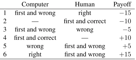
Recall that the non-oracle algorithms were un-aware of the true reward function. To best simulate conventional quiz bowl settings, a correct answer was+10and the incorrect answer was−5. The full payoff matrix for the computer is shown in Table 2.
Cases where the opponent buzzes first but is wrong are equivalent to rapacious classification, as there is no longer any incentive to answer early. Thus we exclude such situations (Outcomes 3, 5, 6 in Table 2) from the dataset to focus on the challenge of process-ing clues incrementally.
Computer Human Payoff
1 first and wrong right −15
2 — first and correct −10
3 first and wrong wrong −5
4 first and correct — +10
5 wrong first and wrong +5
[image:7.612.314.534.150.248.2]6 right first and wrong +15
Table 2: Payoff matrix (from the computer’s perspective) for when agents “buzz” during a question. To focus on incremental classification, we exclude instances where the human interrupts with anincorrect answer, as after an opponent eliminates themselves, the answering reduces to rapacious classification.
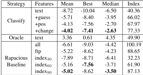
Table 3 shows the algorithm did much better when it had access to the posterior. While incremental algorithms outperform rapacious baselines, they lose to humans. Against the median and average players, they lose between three and four points per question, and nearly twice that against the best players.
Although the content model is simple, this poor performance is not from the content model never producing the correct answer. To see this, we also computed the optimal actions that could be executed. We called this strategy the oracle strategy; it was able to consistently win against its opponents. Thus, while the content model was able to come up with correct answers often enough to on average win against oppo-nents (even the best human players), we were unable to consistently learn winning policies.
There are two ways to solve this problem: create deeper, more nuanced policies (or the features that feed into them) or refine content models that provide the signal needed for our policies to make sound decisions. We chose to refine the content model, as we felt we had added all of the obvious features for learning effective policies.
7 Expanding the Content Model
Strategy Features Mean Best Median Index
Classify
text -8.72 -10.04 -6.50 40.36 +guess -5.71 -8.40 -3.95 66.02 +pos -4.13 -7.56 -2.70 67.97 +change -4.02 -7.41 -2.63 77.33
Oracle text 3.36 0.61 4.35 49.90
all -6.61 -9.03 -4.42 100.19 ftp -5.22 -8.62 -4.23 88.65 Rapacious index30 -7.89 -8.71 -6.41 32.23
Baseline index60 -5.16 -7.56 -3.71 61.90
[image:8.612.70.304.57.180.2]index90 -5.02 -8.62 -3.50 87.13
Table 3: Performance of strategies against users. The human scoring columns show the average points per ques-tion (positive means winning on average, negative means losing on average) that the algorithm would expect to ac-cumulate per question versus each human amalgam metric. The index column notes the average index of the token when the strategy chose to buzz.
of a question, which substantially narrows the an-swer space. Ideally, the content model should con-duct the same calculus—if a question seems to be about mathematics, all answers related with mathe-matics should be more likely in the posterior. This was consistent with our error analysis; many errors were non-sensical (e.g., answering “entropy” for “Jo-hannes Brahms”, when an answer such as “Robert Schumann”, another composer, would be better).
In addition, assuming independence between fea-tures given a label causes us to ignore potentially informative multiword expressions such as quota-tions, titles, or dates. Adding a language model to our content model allows us to capture some of these phenomena.
To create a model that jointly models categories and local context, we propose the following model:
1. Draw a distribution over labelsφ∼Dir(α)
2. Draw a background distribution over words θ0 ∼
Dir(λ0~1)
(a) For each categorycof questions, draw a distribution over wordsθc∼Dir(λ1θ0).
i. For each labellin categoryc, draw a distribu-tion over wordsθl,c∼Dir(λ2θc)
A. For each typev, draw a bigram distribution θl,c,v∼Dir(λ3θl,c)
3. Draw a distribution over labelsφ∼Dir(α).
4. For each question with categorycandN words, draw answerl∼Mult(φ):
(a) Assumew0≡START
(b) Drawwn∼Mult(θl,c,wn−1)forn∈ {1. . . N}
This creates a language model over categories,
la-bels, and observed words (we use “words” loosely, as bigrams replace some word pairs). By constructing the word distributions using hierarchical distributions based on domain and ngrams (a much simpler para-metric version of more elaborate methods (Wood and Teh, 2009)), we can share statistical strength across related contexts. We assume that labels are (only) associated with their majority category as seen in our training data and that category assignments are ob-served. All scaling parametersλwere set to 10,000,
αwas 1.0, and the vocabulary was still 25,000. We used the maximal seating assignment (Wallach, 2008) for propagating counts through the Dirichlet hierarchy. Thus, if the wordvappearedBl,u,vtimes
in labellfollowing a preceding wordu,Sl,vtimes in
labell,Tc,vtimes in categoryc, andGvtimes in total,
we estimate the probability of a wordv appearing in labelk, categoryt, and after worduasp(wn =
v|lab=l,cat=c, wn−1 =u;~λ) =
Bl,u,v+λ3
Sl,v+λ2Tc,v+λ1
Gv+λ0/V G·+λ0 Tc,·+λ2 Sl,·+λ2
Bl,u,·+λ3
, (3)
where we use · to represent marginalization, e.g.
Tc,· =Pv0Tc,v0. As with na¨ıve Bayes, Bayes’ rule provides posterior label probabilities (Equation 2).
We compare the na¨ıve model with models that capture more of the content in the text in Table 4; these results also include intermediate models be-tween na¨ıve Bayes and the full content model: “cat” (omit 2.a.i.A) and “bigram” (omit 2.a). These models perform much better than the na¨ıve Bayes models seen in Table 3. They are about even against the mean and median players and lose four points per question against top players.
7.1 Qualitative Analysis
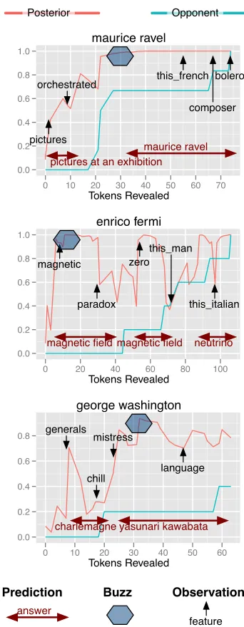
In this section, we explore what defects are prevent-ing the model presented here from competprevent-ing with top players, exposing challenges in reinforcement learning, interpreting pragmatic cues, and large data. Three examples of failures of the model are in Fig-ure 5. This model is the best performing model of the previous section.
Strategy Model Mean Best Median Index
Classify
na¨ıve -4.02 -7.41 -2.63 77.33 cat -1.69 -5.22 0.12 67.97 bigram -3.80 -7.66 -2.51 78.69 bgrm+cat -0.86 -4.46 0.83 63.42
Oracle
naive 3.36 0.61 4.35 49.90
cat 4.48 1.64 5.47 47.88
[image:9.612.73.298.56.158.2]bigram 3.58 0.87 4.61 49.34 bgrm+cat 4.67 1.99 5.74 46.49
Table 4: As in Table 3, performance of strategies against users, but with enhanced content models. Modeling both bigrams and label categories improves overall perfor-mance.
Mussorgsky’s piano piece “Pictures at an Exhibition”. Based on that evidence, the algorithm considers “Pic-tures at an Exhibition” the most likely but does not yet buzz. When it receives enough information to be sure about the correct answer, over half of the players had already buzzed. Correcting this problem would require a more aggressive strategy, perhaps incorpo-rating the identity of the opponent or estimating the difficulty of the question.
Mislead by the Content Model The second ex-ample is a question on Enrico Fermi, an Italian-American physicist. The first clues are about mag-netic fields near a Fermi surface, which causes the content model to view “magnetic field” as the most likely answer. The question’s text, however, has pragmatic cues “this man” and “this Italian” which would have ruled out the abstract answer “magnetic field”. Correcting this would require a model that jointly models content and bigrams (Hardisty et al., 2010), has a coreference system as its content model (Haghighi and Klein, 2007), or determines the correct question type (Moldovan et al., 2000).
Insufficient Data The third example is where our approach had no chance. The question is a very diffi-cult question about George Washington, America’s first president. As a sign of its difficulty, only half the players answered correctly, and only near the end of the question. The question concerns lesser known episodes from Washington’s life, including a mistress caught in the elements. To the content model, of the several hypotheses it considers, the closest match it can find is “Yasunari Kawabata”, who wrote the novelSnow Country, whose plot matches some of these keywords. To answer these types of question,
george washington
Tokens Revealed
0.0 0.2 0.4 0.6 0.8
0 10 20 30 40 50 60
maurice ravel
Tokens Revealed
0.0 0.2 0.4 0.6 0.8 1.0
0 10 20 30 40 50 60 70
enrico fermi
Tokens Revealed 0.0
0.2 0.4 0.6 0.8 1.0
0 20 40 60 80 100
charlemagne yasunari kawabata generals
chill mistress
language magnetic fieldmagnetic field neutrino magnetic
paradox zero
this_man
this_italian pictures
orchestrated
pictures at an exhibition maurice ravel
this_french
composer bolero
Prediction
answer
Observation
feature
Buzz
Posterior Opponent
[image:9.612.339.510.62.502.2]the repository used to train the content model would have to be orders of magnitude larger to be able to link the disparate clues in the question to a consistent target. The content model would also benefit from weighting later (more informative) features higher.
7.2 Assumptions
We have made assumptions to solve a problem that is subtly different that the game of quiz bowl that a human would play. Some of these were simpli-fying assumptions, such as our assumption that the algorithm has a closed set of possible answers (Sec-tion 5.3). Even with this advantage, the algorithm is unable to compete with human players, who choose answers from an unbounded set. On the other hand, to focus on incremental classification, we idealized our human opponents so that they never give incor-rect answers (Section 6). This causes our estimates of our performance to be lower than they would be against real players.
8 Conclusion and Future Work
We make three contributions. First, we introduce a new setting for exploring the problem of incremental classification: trivia games. This problem is intrin-sically interesting because of its varied topics and competitive elements, has a great quantity of stan-dardized, machine-readable data, and also has the boon of being cheaply and easily annotated. We took advantage of that ease and created a framework for quickly and efficiently gathering examples of humans doing incremental classification.
There are other potential uses for the dataset; the progression of clues from obscure nuggets to could help determine how “known” a particular aspect of an entity is (e.g., that William Jennings Bryant gave the “Cross of Gold” speech is better known his resig-nation after the Lusitania sinking, Figure 1). Which could be used in educational settings (Smith et al., 2008) or summarization (Das and Martins, 2007).
The second contribution shows that humans’ incre-mental classification improves state-of-the-art rapa-cious classification algorithms. While other frame-works (Zaidan et al., 2008) have been proposed to incorporate user clues about features, the system de-scribed here provides analogous features without the need for explicit post-hoc reflection, has faster
anno-tation throughput, and is much cheaper.
The problem of answering quiz bowl questions is itself a challenging task that combines issues from language modeling, large data, coreference, and re-inforcement learning. While we do not address all of these problems, our third contribution is a sys-tem that learns a policy in a MDP for incremental classification even in very large state spaces; it can successfully compete with skilled human players.
Incorporating richer content models is one of our next steps. This would allow us to move beyond the closed-set model and use a more general coreference model (Haghighi and Klein, 2007) for identifying answers and broader corpora for training. In addi-tion, using larger corpora would allow us to have more comprehensive doubly-hierarchical language models (Wood and Teh, 2009). We are also inter-ested in adding richer models of opponents to the state space that would adaptively adjust strategies as it learned more about the strengths and weaknesses of its opponent (Waugh et al., 2011).
Further afield, our presentation of sentences closely resembles paradigms for cognitive experi-ments in linguistics (Thibadeau et al., 1982) but are much cheaper to conduct. If online processing ef-fects (Levy et al., 2008; Levy, 2011) could be ob-served in buzzing behavior; e.g., if a confusingly worded phrase depresses buzzing probability, it could help validate cognitively-inspired models of online sentence processing.
Acknowledgments
We thank the many players who played our online quiz bowl to provide our data (and hopefully had fun doing so) and Carlo Angiuli, Arnav Moudgil, and Jerry Vinokurov for providing access to quiz bowl questions. This research was supported by NSF grant #1018625. Jordan Boyd-Graber is also supported by the Army Research Laboratory through ARL Cooper-ative Agreement W911NF-09-2-0072. Any opinions, findings, conclusions, or recommendations expressed are the authors’ and do not necessarily reflect those of the sponsors.
References
Pieter Abbeel and Andrew Y. Ng. 2004. Apprentice-ship learning via inverse reinforcement learning. In Proceedings of International Conference of Machine Learning.
J. Blatz, E. Fitzgerald, G. Foster, S. Gandrabur, C. Goutte, A. Kulesza, A. Sanchis, and N. Ueffing. 2004. Confi-dence estimation for machine translation. In Proceed-ings of the Association for Computational Linguistics. Mark Boddy and Thomas L. Dean. 1989. Solving
time-dependent planning problems. InInternational Joint Conference on Artificial Intelligence, pages 979–984. Morgan Kaufmann Publishers, August.
Nicol`o Cesa-Bianchi, Shai Shalev-Shwartz, and Ohad Shamir. 2011. Efficient learning with partially ob-served attributes. Journal of Machine Learning Re-search, 12:2857–2878.
Xiaoyong Chai, Lin Deng, Qiang Yang, and Charles X. Ling. 2004. Test-cost sensitive naive bayes classi-fication. InIEEE International Conference on Data Mining.
Dipanjan Das and Andre Martins. 2007. A survey on automatic text summarization. Engineering and Tech-nology, 4:192–195.
Hal Daum´e III. 2004. Notes on CG and LM-BFGS optimization of logistic regression. Pa-per available at http://pub.hal3.name/
˜daume04cg-bfgs, implementation available at
http://hal3.name/megam/.
Rong-En Fan, Kai-Wei Chang, Cho-Jui Hsieh, Xiang-Rui Wang, and Chih-Jen Lin. 2008. LIBLINEAR: A library for large linear classification. Journal of Machine Learning Research, 9:1871–1874.
David Ferrucci, Eric Brown, Jennifer Chu-Carroll, James Fan, David Gondek, Aditya A. Kalyanpur, Adam Lally, J. William Murdock, Eric Nyberg, John Prager, Nico Schlaefer, and Chris Welty. 2010. Building Watson:
An Overview of the DeepQA Project. AI Magazine, 31(3).
Aria Haghighi and Dan Klein. 2007. Unsupervised coref-erence resolution in a nonparametric bayesian model. InProceedings of the Association for Computational Linguistics.
Eric Hardisty, Jordan Boyd-Graber, and Philip Resnik. 2010. Modeling perspective using adaptor grammars. InProceedings of Emperical Methods in Natural Lan-guage Processing.
Michael C. Horsch and David Poole. 1998. An anytime algorithm for decision making under uncertainty. In Proceedings of Uncertainty in Artificial Intelligence. Ken Jennings. 2006. Brainiac: adventures in the curious,
competitive, compulsive world of trivia buffs. Villard. Shihao Ji and Lawrence Carin. 2007. Cost-sensitive
fea-ture acquisition and classification.Pattern Recognition, 40:1474–1485, May.
Shyong K. Lam, David M. Pennock, Dan Cosley, and Steve Lawrence. 2003. 1 billion pages = 1 million dollars? mining the web to play ”who wants to be a mil-lionaire?”. InProceedings of Uncertainty in Artificial Intelligence.
John Langford and Bianca Zadrozny. 2005. Relating reinforcement learning performance to classification performance. InProceedings of International Confer-ence of Machine Learning.
Roger P. Levy, Florencia Reali, and Thomas L. Griffiths. 2008. Modeling the effects of memory on human on-line sentence processing with particle filters. In Pro-ceedings of Advances in Neural Information Processing Systems.
Roger Levy. 2011. Integrating surprisal and uncertain-input models in online sentence comprehension: formal techniques and empirical results. InProceedings of the Association for Computational Linguistics.
David D. Lewis. 1998. Naive (Bayes) at forty: The inde-pendence assumption in information retrieval. In Claire N´edellec and C´eline Rouveirol, editors,Proceedings of European Conference of Machine Learning, number 1398.
Michael L. Littman, Greg A. Keim, and Noam Shazeer. 2002. A probabilistic approach to solving crossword puzzles.Artif. Intell., 134(1-2):23–55, January. Edward Loper and Steven Bird. 2002. NLTK: the
natu-ral language toolkit. InTools and methodologies for teaching.
Prem Melville, Maytal Saar-Tsechansky, Foster Provost, and Raymond J. Mooney. 2005. An expected utility approach to active feature-value acquisition. In Inter-national Conference on Data Mining, November. Dan Moldovan, Sanda Harabagiu, Marius Pasca, Rada
Rus. 2000. The structure and performance of an open-domain question answering system. InProceedings of the Association for Computational Linguistics. Joakim Nivre. 2008. Algorithms for deterministic
in-cremental dependency parsing. Comput. Linguist., 34(4):513–553, December.
Jay Pujara, Hal Daume III, and Lise Getoor. 2011. Using classifier cascades for scalable e-mail classification. InCollaboration, Electronic Messaging, Anti-Abuse and Spam Conference, ACM International Conference Proceedings Series.
Sebastian Riedel, David McClosky, Mihai Surdeanu, An-drew McCallum, and Christopher D. Manning. 2011. Model combination for event extraction in bionlp 2011. InProceedings of the BioNLP Workshop.
Afshin Rostamizadeh, Alekh Agarwal, and Peter L. Bartlett. 2011. Learning with missing features. In Proceedings of Uncertainty in Artificial Intelligence. Maytal Saar-Tsechansky and Foster Provost. 2007.
Han-dling missing values when applying classification mod-els. Journal of Machine Learning Research, 8:1623– 1657, December.
Gerard. Salton. 1968. Automatic Information Organiza-tion and Retrieval. McGraw Hill Text.
Burr Settles. 2011. Closing the loop: Fast, interactive semi-supervised annotation with queries on features and instances. InProceedings of Emperical Methods in Natural Language Processing.
David Silver, Richard S. Sutton, and Martin M¨uller. 2008. Sample-based learning and search with permanent and transient memories. In International Conference on Machine Learning.
Noah A. Smith, Michael Heilman, and Rebecca Hwa. 2008. Question generation as a competitive under-graduate course project. InProceedings of the NSF Workshop on the Question Generation Shared Task and Evaluation Challenge.
Umar Syed, Michael Bowling, and Robert E. Schapire. 2008. Apprenticeship learning using linear program-ming. InProceedings of International Conference of Machine Learning.
Gerald Tesauro and Gregory R. Galperin. 1996. On-line policy improvement using monte-carlo search. In Pro-ceedings of Advances in Neural Information Processing Systems.
Robert Thibadeau, Marcel A. Just, and Patricia A. Carpen-ter. 1982. A model of the time course and content of reading.Cognitive Science, 6.
Hanna M Wallach. 2008. Structured Topic Models for Language. Ph.D. thesis, University of Cambridge. Lidan Wang, Donald Metzler, and Jimmy Lin. 2010.
Ranking Under Temporal Constraints. InProceedings of the ACM International Conference on Information and Knowledge Management.
Kevin Waugh, Brian D. Ziebart, and J. Andrew Bagnell. 2011. Computational rationalization: The inverse equi-librium problem. InProceedings of International Con-ference of Machine Learning.
F. Wood and Y. W. Teh. 2009. A hierarchical nonpara-metric Bayesian approach to statistical language model domain adaptation. InProceedings of Artificial Intelli-gence and Statistics.
Omar F. Zaidan, Jason Eisner, and Christine Piatko. 2008. Machine learning with annotator rationales to reduce annotation cost. In Proceedings of the NIPS*2008 Workshop on Cost Sensitive Learning.