Learning Syntactic Categories Using Paradigmatic Representations of Word Context

Learning Syntactic Categories Using Paradigmatic Representations of

Word Context

Mehmet Ali Yatbaz Enis Sert Deniz Yuret

Artificial Intelligence Laboratory Koc¸ University, ˙Istanbul, Turkey {myatbaz,esert,dyuret}@ku.edu.tr

Abstract

We investigate paradigmatic representations of word context in the domain of unsupervised syntactic category acquisition. Paradigmatic representations of word context are based on potential substitutes of a word in contrast to syntagmatic representations based on prop-erties of neighboring words. We compare a bigram based baseline model with several paradigmatic models and demonstrate signif-icant gains in accuracy. Our best model based on Euclidean co-occurrence embedding com-bines the paradigmatic context representation with morphological and orthographic features and achieves 80% many-to-one accuracy on a 45-tag 1M word corpus.

1 Introduction

Grammar rules apply not to individual words (e.g. dog, eat) but to syntactic categories of words (e.g. noun, verb). Thus constructing syntactic categories (also known as lexical or part-of-speech categories) is one of the fundamental problems in language ac-quisition.

Syntactic categories represent groups of words that can be substituted for one another without alter-ing the grammaticality of a sentence. Lalter-inguists iden-tify syntactic categories based on semantic, syntac-tic, and morphological properties of words. There is also evidence that children use prosodic and phono-logical features to bootstrap syntactic category ac-quisition (Ambridge and Lieven, 2011). However there is as yet no satisfactory computational model that can match human performance. Thus

identify-ing the best set of features and best learnidentify-ing algo-rithms for syntactic category acquisition is still an open problem.

Relationships between linguistic units can be classified into two types: syntagmatic (concerning positioning), and paradigmatic (concerning substitu-tion). Syntagmatic relations determine which units can combine to create larger groups and paradig-matic relations determine which units can be sub-stituted for one another. Figure 1 illustrates the paradigmatic vs syntagmatic axes for words in a simple sentence and their possible substitutes.

In this study, we represent the paradigmatic axis directly by buildingsubstitute vectorsfor each word position in the text. The dimensions of a substi-tute vector represent words in the vocabulary, and the magnitudes represent the probability of occur-rence in the given position. Note that the substitute vector for a word position (e.g. the second word in Fig. 1) is a function of the context only (i.e. “the cried”), and does not depend on the word that does actually appear there (i.e. “man”). Thus

substi-Figure 1: Syntagmatic vs. paradigmatic axes for words in a simple sentence (Chandler, 2007).

tute vectors representindividual word contexts, not word types. We refer to the use of features based on substitute vectors asparadigmatic representations of word context.

Our preliminary experiments indicated that using context information alone without the identity or the features of the target word (e.g. using dimension-ality reduction and clustering on substitute vectors) has limited success and modeling the co-occurrence of word and context types is essential for inducing syntactic categories. In the models presented in this paper, we combine paradigmatic representations of word context with features of co-occurring words within the co-occurrence data embedding (CODE) framework (Globerson et al., 2007; Maron et al., 2010). The resulting embeddings for word types are split into 45 clusters using k-means and the clusters are compared to the 45 gold tags in the 1M word Penn Treebank Wall Street Journal corpus (Mar-cus et al., 1999). We obtain many-to-one accura-cies up to .7680 using only distributional informa-tion (the identity of the word and a representainforma-tion of its context) and .8023 using morphological and or-thographic features of words improving the state-of-the-art in unsupervised part-of-speech tagging per-formance.

The high probability substitutes reflect both se-mantic and syntactic properties of the context as seen in the example below (the numbers in paren-theses give substitute probabilities):

“Pierre Vinken, 61 years old, will join the board as a nonexecutive director Nov. 29.”

the:its (.9011), the (.0981), a (.0006),. . . board: board (.4288), company (.2584), firm (.2024), bank (.0731),. . .

Top substitutes for the word “the” consist of words that can act as determiners. Top substitutes for “board” are not only nouns, but specifically nouns compatible with the semantic context.

This example illustrates two concerns inherent in all distributional methods: (i) words that are gener-ally substitutable like “the” and “its” are placed in separate categories (DT andPRP$) by the gold stan-dard, (ii) words that are generally not substitutable like “do” and “put” are placed in the same category

(VB). Freudenthal et al. (2005) point out that cat-egories with unsubstitutable words fail the standard linguistic definition of a syntactic category and chil-dren do not seem to make errors of substituting such words in utterances (e.g. “What do you want?” vs. *“What put you want?”). Whether gold standard part-of-speech tags or distributional categories are better suited to applications like parsing or machine translation can be best decided using extrinsic eval-uation. However in this study we follow previous work and evaluate our results by comparing them to gold standard part-of-speech tags.

Section 2 gives a detailed review of related work. Section 3 describes the dataset and the construction of the substitute vectors. Section 4 describes co-occurrence data embedding, the learning algorithm used in our experiments. Section 5 describes our experiments and compares our results with previ-ous work. Section 6 gives a brief error analysis and Section 7 summarizes our contributions. All the data and the code to replicate the results given in this paper is available from the authors’ website at http://goo.gl/RoqEh.

2 Related Work

There are several good reviews of algorithms for unsupervised part-of-speech induction (Christodoulopoulos et al., 2010; Gao and Johnson, 2008) and models of syntactic category acquisition (Ambridge and Lieven, 2011).

This work is to be distinguished from supervised part-of-speech disambiguation systems, which use labeled training data (Church, 1988), unsupervised disambiguation systems, which use a dictionary of possible tags for each word (Merialdo, 1994), or prototype driven systems which use a small set of prototypes for each class (Haghighi and Klein, 2006). The problem of induction is important for studying under-resourced languages that lack la-beled corpora and high quality dictionaries. It is also essential in modeling child language acquisition be-cause every child manages to induce syntactic cat-egories without access to labeled sentences, labeled prototypes, or dictionary constraints.

types and their context statistics. Word-feature mod-els incorporate additional morphological and ortho-graphic features.

2.1 Distributional models

Distributional models can be further categorized into three subgroups based on the learning algorithm. The first subgroup represents each word type with its context vector and clusters these vectors accordingly (Sch¨utze, 1995). Work in modeling child syntac-tic category acquisition has generally followed this clustering approach (Redington et al., 1998; Mintz, 2003). The second subgroup consists of proba-bilistic models based on the Hidden Markov Model (HMM) framework (Brown et al., 1992). A third group of algorithms constructs a low dimensional representation of the data that represents the empir-ical co-occurrence statistics of word types (Glober-son et al., 2007), which is covered in more detail in Section 4.

Clustering: Clustering based methods represent context using neighboring words, typically a sin-gle word on the left and a sinsin-gle word on the right called a “frame” (e.g.,thedogis;thecatis). They cluster word types rather than word tokens based on the frames they occupy thus employing one-tag-per-word assumption from the beginning (with the ex-ception of some methods in (Sch¨utze, 1995)). They may suffer from data sparsity caused by infrequent words and infrequent contexts. The solutions sug-gested either restrict the set of words and set of con-texts to be clustered to the most frequently observed, or use dimensionality reduction. Redington et al. (1998) define context similarity based on the num-ber of common frames bypassing the data sparsity problem but achieve mediocre results. Mintz (2003) only uses the most frequent 45 frames and Biemann (2006) clusters the most frequent 10,000 words us-ing contexts formed from the most frequent 150-200 words. Sch¨utze (1995) and Lamar et al. (2010b) employ SVD to enhance similarity between less fre-quently observed words and contexts. Lamar et al. (2010a) represent each context by the currently as-signed left and right tag (which eliminates data spar-sity) and cluster word types using a soft k-means style iterative algorithm. They report the best clus-tering result to date of .708 many-to-one accuracy

on a 45-tag 1M word corpus.

HMMs: The prototypical bitag HMM model max-imizes the likelihood of the corpus w1. . . wn

expressed as P(w1|c1)

Qn

i=2P(wi|ci)P(ci|ci−1)

wherewi are the word tokens andci are their

(hid-den) tags. One problem with such a model is its ten-dency to distribute probabilities equally and the re-sulting inability to model highly skewed word-tag distributions observed in hand-labeled data (John-son, 2007). To favor sparse word-tag distributions one can enforce a strict one-tag-per-word solution (Brown et al., 1992; Clark, 2003), use sparse pri-ors in a Bayesian setting (Goldwater and Griffiths, 2007; Johnson, 2007), or use posterior regulariza-tion (Ganchev et al., 2010). Each of these techniques provide significant improvements over the standard HMM model: for example Gao and Johnson (2008) show that sparse priors can gain from 4% (.62 to .66 with a 1M word corpus) in cross-validated many-to-one accuracy. However Christodoulopoulos et al. (2010) show that the older one-tag-per-word models such as (Brown et al., 1992) outperform the more sophisticated sparse prior and posterior regulariza-tion methods both in speed and accuracy (the Brown model gets .68 many-to-one accuracy with a 1M word corpus). Given that close to 95% of the word occurrences in human labeled data are tagged with their most frequent part of speech (Lee et al., 2010), this is probably not surprising; one-tag-per-word is a fairly good first approximation for induction.

2.2 Word-feature models

in-duced prototypes and report an 8% improvement over the baseline Brown model. Christodoulopou-los et al. (2011) define a type-based Bayesian multi-nomial mixture model in which each word instance is generated from the corresponding word type mix-ture component and word contexts are represented as features. They achieve a .728 MTO score by ex-tending their model with additional morphological and alignment features gathered from parallel cor-pora. To our knowledge, nobody has yet tried to incorporate phonological or prosodic features in a computational model for syntactic category acquisi-tion.

2.3 Paradigmatic representations

Sahlgren (2006) gives a detailed analysis of paradig-matic and syntagparadig-matic relations in the context of word-space models used to represent word mean-ing. Sahlgren’s paradigmatic model represents word types using co-occurrence counts of their frequent neighbors, in contrast to his syntagmatic model that represents word types using counts of contexts (doc-uments, sentences) they occur in. Our substitute vectors do not represent word types at all, but con-texts of word tokensusing probabilities of likely sub-stitutes. Sahlgren finds that in word-spaces built by frequent neighbor vectors, more nearest neighbors share the same part-of-speech compared to word-spaces built by context vectors. We find that rep-resenting the paradigmatic axis more directly using substitute vectors rather than frequent neighbors im-prove part-of-speech induction.

Our paradigmatic representation is also related to the second order co-occurrences used in (Sch¨utze, 1995). Sch¨utze concatenates the left and right text vectors for the target word type with the left text vector of the right neighbor and the right con-text vector of the left neighbor. The vectors from the neighbors include potential substitutes. Our method improves on his foundation by using a 4-gram lan-guage model rather than bigram statistics, using the whole 78,498 word vocabulary rather than the most frequent 250 words. More importantly, rather than simply concatenating vectors that represent the tar-get word with vectors that represent the context we use S-CODE to model their co-occurrence statistics.

2.4 Evaluation

We report many-to-one and V-measure scores for our experiments as suggested in (Christodoulopou-los et al., 2010). The many-to-one (MTO) evaluation maps each cluster to its most frequent gold tag and reports the percentage of correctly tagged instances. The MTO score naturally gets higher with increas-ing number of clusters but it is an intuitive met-ric when comparing results with the same number of clusters. The V-measure (VM) (Rosenberg and Hirschberg, 2007) is an information theoretic met-ric that reports the harmonic mean of homogeneity (each cluster should contain only instances of a sin-gle class) and completeness (all instances of a class should be members of the same cluster). In Sec-tion 6 we argue that homogeneity is perhaps more important in part-of-speech induction and suggest MTO with a fixed number of clusters as a more in-tuitive metric.

3 Substitute Vectors

In this study, we predict the part of speech of a word in a given context based on its substitute vector. The dimensions of the substitute vector represent words in the vocabulary, and the entries in the substitute vector represent the probability of those words be-ing used in the given context. Note that the substi-tute vector is a function of the context only and is indifferent to the target word. This section details the choice of the data set, the vocabulary and the es-timation of substitute vector probabilities.

cor-pus is 96.

It is best to use both left and right context when estimating the probabilities for potential lexical sub-stitutes. For example, in“He lived in San Francisco suburbs.”, the tokenSanwould be difficult to guess from the left context but it is almost certain look-ing at the right context. We definecwas the2n−1

word window centered around the target word posi-tion: w−n+1. . . w0. . . wn−1 (n = 4 is the n-gram

order). The probability of a substitute wordwin a given contextcwcan be estimated as:

P(w0 =w|cw) ∝ P(w−n+1. . . w0. . . wn−1)(1)

= P(w−n+1)P(w−n+2|w−n+1)

. . . P(wn−1|wn−−n+12 ) (2)

≈ P(w0|w−n−1+1)P(w1|w0−n+2)

. . . P(wn−1|wn−0 2) (3)

where w_ij represents the sequence of words

wiwi+1. . . wj. In Equation 1, P(w|cw) is

pro-portional toP(w−n+1. . . w0. . . wn+1)because the

words of the context are fixed. Terms without w0

are identical for each substitute in Equation 2 there-fore they have been dropped in Equation 3. Finally, because of the Markov property of n-gram language model, only the closestn−1words are used in the experiments.

Near the sentence boundaries the appropriate terms were truncated in Equation 3. Specifically, at the beginning of the sentence shorter n-gram con-texts were used and at the end of the sentence terms beyond the end-of-sentence token were dropped.

For computational efficiency only the top 100 substitutes and their unnormalized probabilities were computed for each of the 1,173,766 positions in the test set1. The probability vectors for each po-sition were normalized to add up to 1.0 giving us the final substitute vectors used in the rest of this study.

1

The substitutes with unnormalized log probabilities can be downloaded fromhttp://goo.gl/jzKH0. For a descrip-tion of theFASTSUBSalgorithm used to generate the substitutes please see http://arxiv.org/abs/1205.5407v1. FASTSUBS accomplishes this task in about 5 hours, a naive algorithm that looks at the whole vocabulary would take more than 6 days on a typical 2012 workstation.

4 Co-occurrence Data Embedding

The general strategy we follow for unsupervised syntactic category acquisition is to combine features of the context with the identity and features of the target word. Our preliminary experiments indicated that using the context information alone (e.g. clus-tering substitute vectors) without the target word identity and features had limited success.2 It is the co-occurrence of a target word with a particular type of context that best predicts the syntactic category. In this section we review the unsupervised meth-ods we used to model co-occurrence statistics: the Co-occurrence Data Embedding (CODE) method (Globerson et al., 2007) and its spherical extension (S-CODE) introduced by (Maron et al., 2010).

LetXandY be two categorical variables with fi-nite cardinalities|X|and|Y|. We observe a set of pairs{xi, yi}ni=1 drawn IID from the joint

distribu-tion ofXandY. The basic idea behind CODE and related methods is to represent (embed) each value ofX and each value of Y as points in a common low dimensional Euclidean spaceRdsuch that val-ues that frequently co-occur lie close to each other. There are several ways to formalize the relationship between the distances and co-occurrence statistics, in this paper we use the following:

p(x, y) = 1

Zp¯(x)¯p(y)e −d2

x,y ₍₄₎

whered2

x,y is the squared distance between the

em-beddings of x andy, p¯(x) and p¯(y) are empirical probabilities, and Z = P

x,yp¯(x)¯p(y)e −d2

x,y _{is a}

normalization term. If we use the notation φx for

the point corresponding to x and ψy for the point corresponding toy thend2_x,y = kφx −ψyk2_{. The}

log-likelihood of a given embedding`(φ, ψ)can be

2

expressed as:

`(φ, ψ) =X x,y

¯

p(x, y) logp(x, y) (5)

=X

x,y ¯

p(x, y)(−logZ+ log ¯p(x)¯p(y)−d2_x,y)

=−logZ+const−X

x,y ¯

p(x, y)d2_x,y

The likelihood is not convex in φ andψ. We use gradient ascent to find an approximate solution for a set ofφx, ψy that maximize the likelihood. The

gradient of the d2_x,y term pulls neighbors closer in proportion to the empirical joint probability:

∂ ∂φx

X

x,y

−p¯(x, y)d2_x,y =X y

2¯p(x, y)(ψy−φx)

(6) The gradient of theZ term pushes neighbors apart in proportion to the estimated joint probability:

∂ ∂φx

(−logZ) =X y

2p(x, y)(φx−ψy) (7)

Thus the net effect is to pull pairs together if their estimated probability is less than the empirical prob-ability and to push them apart otherwise. The gradi-ents with respect toψyare similar.

S-CODE (Maron et al., 2010) additionally re-stricts allφx andψy to lie on the unit sphere. With

this restriction, Z stays around a fixed value dur-ing gradient ascent. This allows S-CODE to sub-stitute an approximate constantZ˜in gradient calcu-lations for the real Z for computational efficiency. In our experiments, we used S-CODE with its sam-pling based stochastic gradient ascent algorithm and smoothly decreasing learning rate.

5 Experiments

In this section we present experiments that evaluate substitute vectors as representations of word con-text within the S-CODE framework. Section 5.1 replicates the bigram based S-CODE results from (Maron et al., 2010) as a baseline. The S-CODE algorithm works with discrete inputs. The substi-tute vectors as described in Section 3 are high di-mensional and continuous. We experimented with two approaches to use substitute vectors in a dis-crete setting. Section 5.2 presents an algorithm that

partitions the high dimensional space of substitute vectors into small neighborhoods and uses the par-tition id as a discrete context representation. Sec-tion 5.3 presents an even simpler model which pairs each word with a random substitute. When the left-word – right-left-word pairs used in the bigram model are replaced with word – partition-id or word – sub-stitute pairs we see significant gains in accuracy. These results support our running hypothesis that paradigmatic features, i.e. potential substitutes of a word, are better determiners of syntactic category compared to left and right neighbors. Section 5.4 explores morphologic and orthographic features as additional sources of information and its results im-prove the state-of-the-art in the field of unsupervised syntactic category acquisition.

Each experiment was repeated 10 times with dif-ferent random seeds and the results are reported with standard errors in parentheses or error bars in graphs. Table 1 summarizes all the results reported in this paper and the ones we cite from the literature.

5.1 Bigram model

In (Maron et al., 2010) adjacent word pairs (bi-grams) in the corpus are fed into the S-CODE algo-rithm asX, Y samples. The algorithm uses stochas-tic gradient ascent to find theφx, ψyembeddings for

left and right words in these bigrams on a single 25-dimensional sphere. At the end each wordwin the vocabulary ends up with two points on the sphere, a φw point representing the behavior of w as the left word of a bigram and aψw point representing

it as the right word. The two vectors forware con-catenated to create a 50-dimensional representation at the end. These 50-dimensional vectors are clus-tered using an instance weighted k-means algorithm and the resulting groups are compared to the cor-rect part-of-speech tags. Maron et al. (2010) report many-to-one scores of .6880 (.0016) for 45 clusters and .7150 (.0060) for 50 clusters (on the full PTB45 tag-set). If only φw vectors are clustered without concatenation we found the performance drops sig-nificantly to about .62.

Distributional Models MTO VM (Lamar et al., 2010a) .708 -(Brown et al., 1992)* .678 .630 (Goldwater et al., 2007) .632 .562 (Ganchev et al., 2010)* .625 .548 (Maron et al., 2010) .688 (.0016)

-Bigrams (Sec. 5.1) .7314 (.0096) .6558 (.0052) Partitions (Sec. 5.2) .7554 (.0055) .6703 (.0037) Substitutes (Sec. 5.3) .7680 (.0038) .6822 (.0029)

Models with Additional Features MTO VM

(Clark, 2003)* .712 .655

(Christodoulopoulos et al., 2011) .728 .661 (Berg-Kirkpatrick and Klein, 2010) .755 -(Christodoulopoulos et al., 2010) .761 .688 (Blunsom and Cohn, 2011) .775 .697 Substitutes and Features (Sec. 5.4) .8023 (.0070) .7207 (.0041)

Table 1: Summary of results in terms of the MTO and VM scores. Standard errors are given in parentheses when available. Starred entries have been reported in the review paper (Christodoulopoulos et al., 2010). Distributional models use only the identity of the target word and its context. The models on the right incorporate orthographic and morphological features.

was kept with its original capitalization, (ii) the learning rate parameters were adjusted to ϕ0 =

50, η0 = 0.2 for faster convergence in log

likeli-hood, (iii) the number of s-code iterations were in-creased from 12 to 50 million, (iv) k-means initial-ization was improved using (Arthur and Vassilvit-skii, 2007), and (v) the number of k-means restarts were increased to 128 to improve clustering and re-duce variance.

5.2 Random partitions

Instead of using left-word – right-word pairs as in-puts to S-CODE we wanted to pair each word with a paradigmatic representation of its context to get a di-rect comparison of the two context representations. To obtain a discrete representation of the context, the random–partitions algorithm first designates a random subset of substitute vectors as centroids to partition the space, and then associates each context with the partition defined by the closest centroid in cosine distance. Each partition thus defined gets a unique id, and word (X) – partition-id (Y) pairs are given to S-CODE as input. The algorithm cycles through the data until we get approximately 50 mil-lion updates. The resultingφx vectors are clustered

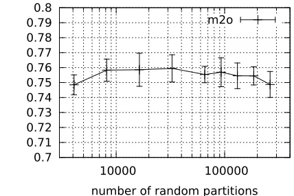
using the k-means algorithm (no vector concatena-tion is necessary). Using default settings (64K ran-dom partitions, 25 s-code dimensions,Z = 0.166) the many-to-one accuracy is .7554 (.0055) and the V-measure is .6703 (.0037).

To analyze the sensitivity of this result to our spe-cific parameter settings we ran a number of experi-ments where each parameter was varied over a range of values.

Figure 2 gives results where the number of initial

0.7 0.71 0.72 0.73 0.74 0.75 0.76 0.77 0.78 0.79 0.8

10000 100000

number of random partitions m2o

Figure 2: MTO is not sensitive to the number of partitions used to discretize the substitute vector space within our experimental range.

random partitions is varied over a large range and shows the results to be fairly stable across two orders of magnitude.

Figure 3 shows that at least 10 embedding dimen-sions are necessary to get within 1% of the best re-sult, but there is no significant gain from using more than 25 dimensions.

0.35 0.4 0.45 0.5 0.55 0.6 0.65 0.7 0.75 0.8

1 10 100

number of s-code dimensions m2o

Figure 3: MTO falls sharply for less than 10 S-CODE dimensions, but more than 25 do not help.

0.7 0.71 0.72 0.73 0.74 0.75 0.76 0.77 0.78 0.79 0.8

0.01 0.1 1

s-code Z approximation m2o

Figure 4: MTO is fairly stable as long as theZ˜constant is within an order of magnitude of the realZvalue.

ing.

We find the random partition algorithm to be fairly robust to different parameter settings and the resulting many-to-one score significantly better than the bigram baseline.

5.3 Random substitutes

Another way to use substitute vectors in a dis-crete setting is simply to sample individual substi-tute words from them. The random-substisubsti-tutes al-gorithm cycles through the test data and pairs each word with a random substitute picked from the pre-computed substitute vectors (see Section 3). We ran the random-substitutes algorithm to generate 14 mil-lion word (X) – random-substitute (Y) pairs (12 substitutes for each token) as input to S-CODE. Clustering the resulting φx vectors yields a

many-to-one score of .7680 (.0038) and a V-measure of

.6822 (.0029).

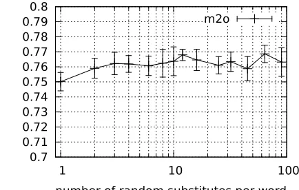
This result is close to the previous result by the random-partition algorithm, .7554 (.0055), demon-strating that two very different discrete represen-tations of context based on paradigmatic features give consistent results. Both results are significantly above the bigram baseline, .7314 (.0096). Figure 5 illustrates that the random-substitute result is fairly robust as long as the training algorithm can observe more than a few random substitutes per word.

0.7 0.71 0.72 0.73 0.74 0.75 0.76 0.77 0.78 0.79 0.8

1 10 100

number of random substitutes per word m2o

Figure 5: MTO is not sensitive to the number of random substitutes sampled per word token.

5.4 Morphological and orthographic features

Clark (2003) demonstrates that using morpholog-ical and orthographic features significantly im-proves part-of-speech induction with an HMM based model. Section 2 describes a number other ap-proaches that show similar improvements. This sec-tion describes one way to integrate addisec-tional fea-tures to the random-substitute model.

The orthographic features we used are similar to the ones in (Berg-Kirkpatrick et al., 2010) with small modifications:

• Initial-Capital: this feature is generated for cap-italized words with the exception of sentence initial words.

• Number: this feature is generated when the to-ken starts with a digit.

• Initial-Apostrophe: this feature is generated for tokens that start with an apostrophe.

We generated morphological features using the unsupervised algorithm Morfessor (Creutz and La-gus, 2005). Morfessor was trained on the WSJ sec-tion of the Penn Treebank using default settings, and a perplexity threshold of 300. The program induced 5 suffix types that are present in a total of 10,484 word types. These suffixes were input to S-CODE as morphological features whenever the associated word types were sampled.

In order to incorporate morphological and ortho-graphic features into S-CODE we modified its in-put. For each word – random-substitute pair gen-erated as in the previous section, we added word – feature pairs to the input for each morphological and orthographic feature of the word. Words on average have 0.25 features associated with them. This in-creased the number of pairs input to S-CODE from 14.1 million (12 substitutes per word) to 17.7 mil-lion (additional 0.25 features on average for each of the 14.1 million words).

Using similar training settings as the previous section, the addition of morphological and ortho-graphic features increased the many-to-one score of the random-substitute model to .8023 (.0070) and V-measure to .7207 (.0041). Both these results im-prove the state-of-the-art in part-of-speech induction significantly as seen in Table 1.

6 Error Analysis

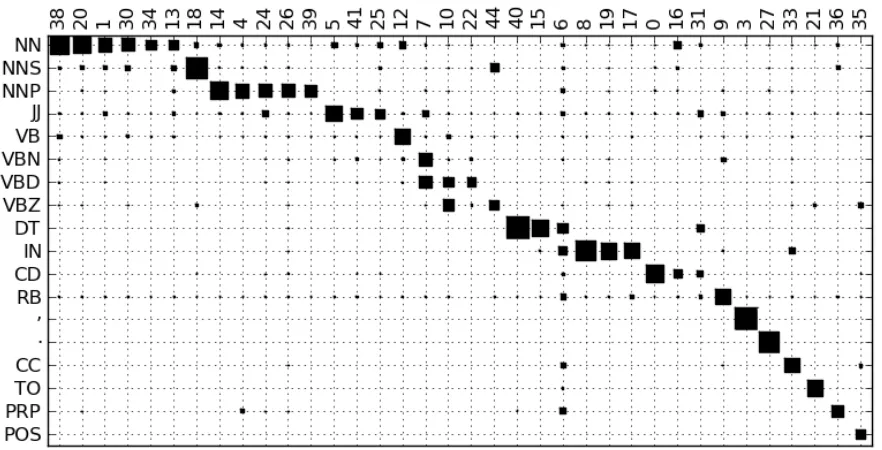
Figure 6 is the Hinton diagram showing the rela-tionship between the most frequent tags and clusters from the experiment in Section 5.4. In general the errors seem to be the lack of completeness (multi-ple large entries in a row), rather than lack of ho-mogeneity (multiple large entries in a column). The algorithm tends to split large word classes into sev-eral clusters. Some examples are:

• Titles like Mr., Mrs., and Dr. are split from the rest of the proper nouns in cluster (39).

• Auxiliary verbs (10) and the verb “say” (22) have been split from the general verb clusters (12) and (7).

• Determiners “the” (40), “a” (15), and capital-ized “The”, “A” (6) have been split into their own clusters.

• Prepositions “of” (19), and “by”, “at” (17) have been split from the general preposition cluster (8).

Nevertheless there are some homogeneity errors as well:

• The adjective cluster (5) also has some noun members probably due to the difficulty of sep-arating noun-noun compounds from adjective modification.

• Cluster (6) contains capitalized words that span a number of categories.

Most closed-class items are cleanly separated into their own clusters as seen in the lower right hand corner of the diagram. The completeness errors are not surprising given that the words that have been split are not generally substitutable with the other members of their Penn Treebank category. Thus it can be argued that metrics that emphasize homo-geneity such as MTO are more appropriate in this context than metrics that average homogeneity and completeness such as VM as long as the number of clusters is controlled.

7 Contributions

Our main contributions can be summarized as fol-lows:

• We introduced substitute vectors as paradig-matic representations of word context and demonstrated their use in syntactic category ac-quisition.

• We demonstrated that using paradigmatic rep-resentations of word context and modeling co-occurrences of word and context types with the S-CODE learning framework give superior results when compared to a baseline bigram model.

Figure 6: Hinton diagram comparing most frequent tags and clusters.

• All our code and data, including the sub-stitute vectors for the one million word Penn Treebank Wall Street Journal dataset, is available at the authors’ website at http://goo.gl/RoqEh.

References

B. Ambridge and E.V.M. Lieven, 2011. Child Language Acquisition: Contrasting Theoretical Approaches, chapter 6.1. Cambridge University Press.

D. Arthur and S. Vassilvitskii. 2007. k-means++: The advantages of careful seeding. In Proceedings of the eighteenth annual ACM-SIAM symposium on Discrete algorithms, pages 1027–1035. Society for Industrial and Applied Mathematics.

Taylor Berg-Kirkpatrick and Dan Klein. 2010. Phyloge-netic grammar induction. InProceedings of the 48th Annual Meeting of the Association for Computational Linguistics, pages 1288–1297, Uppsala, Sweden, July. Association for Computational Linguistics.

Taylor Berg-Kirkpatrick, Alexandre Bouchard-Cˆot´e, John DeNero, and Dan Klein. 2010. Painless unsu-pervised learning with features. InHuman Language Technologies: The 2010 Annual Conference of the North American Chapter of the Association for Com-putational Linguistics, pages 582–590, Los Angeles, California, June. Association for Computational Lin-guistics.

C. Biemann. 2006. Unsupervised part-of-speech tagging employing efficient graph clustering. InProceedings

of the 21st International Conference on computational Linguistics and 44th Annual Meeting of the Associa-tion for ComputaAssocia-tional Linguistics: Student Research Workshop, pages 7–12. Association for Computational Linguistics.

Phil Blunsom and Trevor Cohn. 2011. A hierarchi-cal pitman-yor process hmm for unsupervised part of speech induction. InProceedings of the 49th Annual Meeting of the Association for Computational Linguis-tics: Human Language Technologies, pages 865–874, Portland, Oregon, USA, June. Association for Compu-tational Linguistics.

Peter F. Brown, Peter V. deSouza, Robert L. Mercer, Vin-cent J. Della Pietra, and Jenifer C. Lai. 1992. Class-based n-gram models of natural language. Comput. Linguist., 18:467–479, December.

D. Chandler. 2007. Semiotics: the basics. The Basics Series. Routledge.

Christos Christodoulopoulos, Sharon Goldwater, and Mark Steedman. 2010. Two decades of unsupervised pos induction: how far have we come? InProceedings of the 2010 Conference on Empirical Methods in Nat-ural Language Processing, EMNLP ’10, pages 575– 584, Stroudsburg, PA, USA. Association for Compu-tational Linguistics.

Kenneth Ward Church. 1988. A stochastic parts pro-gram and noun phrase parser for unrestricted text. In

Proceedings of the second conference on Applied nat-ural language processing, ANLC ’88, pages 136–143, Stroudsburg, PA, USA. Association for Computational Linguistics.

Alexander Clark. 2003. Combining distributional and morphological information for part of speech induc-tion. In Proceedings of the tenth conference on Eu-ropean chapter of the Association for Computational Linguistics - Volume 1, EACL ’03, pages 59–66, Stroudsburg, PA, USA. Association for Computational Linguistics.

Mathias Creutz and Krista Lagus. 2005. Inducing the morphological lexicon of a natural language from unannotated text. In Proceedings of AKRR’05, Inter-national and Interdisciplinary Conference on Adap-tive Knowledge Representation and Reasoning, pages 106–113, Espoo, Finland, June.

D. Freudenthal, J.M. Pine, and F. Gobet. 2005. On the resolution of ambiguities in the extraction of syntactic categories through chunking. Cognitive Systems Re-search, 6(1):17–25.

Kuzman Ganchev, Jo˜ao Grac¸a, Jennifer Gillenwater, and Ben Taskar. 2010. Posterior regularization for struc-tured latent variable models. J. Mach. Learn. Res., 99:2001–2049, August.

Jianfeng Gao and Mark Johnson. 2008. A comparison of bayesian estimators for unsupervised hidden markov model pos taggers. InProceedings of the Conference on Empirical Methods in Natural Language Process-ing, EMNLP ’08, pages 344–352, Stroudsburg, PA, USA. Association for Computational Linguistics. Amir Globerson, Gal Chechik, Fernando Pereira, and

Naftali Tishby. 2007. Euclidean embedding of co-occurrence data. J. Mach. Learn. Res., 8:2265–2295, December.

Sharon Goldwater and Tom Griffiths. 2007. A fully bayesian approach to unsupervised part-of-speech tag-ging. In Proceedings of the 45th Annual Meeting of the Association of Computational Linguistics, pages 744–751, Prague, Czech Republic, June. Association for Computational Linguistics.

David Graff, Roni Rosenfeld, and Doug Paul. 1995. Csr-iii text. Linguistic Data Consortium, Philadelphia. Aria Haghighi and Dan Klein. 2006. Prototype-driven

learning for sequence models. In Proceedings of the main conference on Human Language Technology Conference of the North American Chapter of the As-sociation of Computational Linguistics, HLT-NAACL ’06, pages 320–327, Stroudsburg, PA, USA. Associa-tion for ComputaAssocia-tional Linguistics.

Mark Johnson. 2007. Why doesn’t EM find good HMM POS-taggers? InProceedings of the 2007 Joint

Conference on Empirical Methods in Natural guage Processing and Computational Natural Lan-guage Learning (EMNLP-CoNLL), pages 296–305, Prague, Czech Republic, June. Association for Com-putational Linguistics.

Michael Lamar, Yariv Maron, and Elie Bienenstock. 2010a. Latent-descriptor clustering for unsupervised pos induction. InProceedings of the 2010 Conference on Empirical Methods in Natural Language Process-ing, EMNLP ’10, pages 799–809, Stroudsburg, PA, USA. Association for Computational Linguistics. Michael Lamar, Yariv Maron, Mark Johnson, and Elie

Bienenstock. 2010b. Svd and clustering for unsuper-vised pos tagging. In Proceedings of the ACL 2010 Conference Short Papers, pages 215–219, Uppsala, Sweden, July. Association for Computational Linguis-tics.

Yoong Keok Lee, Aria Haghighi, and Regina Barzilay. 2010. Simple type-level unsupervised pos tagging. In Proceedings of the 2010 Conference on Empirical Methods in Natural Language Processing, EMNLP ’10, pages 853–861, Stroudsburg, PA, USA. Associ-ation for ComputAssoci-ational Linguistics.

Mitchell P. Marcus, Beatrice Santorini, Mary Ann Marcinkiewicz, and Ann Taylor. 1999. Treebank-3. Linguistic Data Consortium, Philadelphia.

Yariv Maron, Michael Lamar, and Elie Bienenstock. 2010. Sphere embedding: An application to part-of-speech induction. In J. Lafferty, C. K. I. Williams, J. Shawe-Taylor, R.S. Zemel, and A. Culotta, editors,

Advances in Neural Information Processing Systems 23, pages 1567–1575.

Bernard Merialdo. 1994. Tagging english text with a probabilistic model. Comput. Linguist., 20:155–171, June.

T.H. Mintz. 2003. Frequent frames as a cue for gram-matical categories in child directed speech. Cognition, 90(1):91–117.

M. Redington, N. Crater, and S. Finch. 1998. Distribu-tional information: A powerful cue for acquiring syn-tactic categories. Cognitive Science, 22(4):425–469. A. Rosenberg and J. Hirschberg. 2007. V-measure: A

conditional entropy-based external cluster evaluation measure. InProceedings of the 2007 Joint Conference on Empirical Methods in Natural Language Process-ing and Computational Natural Language LearnProcess-ing, pages 410–420.

Magnus Sahlgren. 2006. The Word-Space Model: Us-ing distributional analysis to represent syntagmatic and paradigmatic relations between words in high-dimensional vector spaces. Ph.D. thesis, Stockholm University.

on European chapter of the Association for Compu-tational Linguistics, EACL ’95, pages 141–148, San Francisco, CA, USA. Morgan Kaufmann Publishers Inc.