Approximate Scalable Bounded Space Sketch for Large Data NLP

Approximate Scalable Bounded Space Sketch for Large Data NLP

Amit Goyal and Hal Daum´e III Dept. of Computer Science

University of Maryland College Park, MD 20742 {amit,hal}@umiacs.umd.edu

Abstract

We exploit sketch techniques, especially the Count-Min sketch, a memory, and time effi-cient framework which approximates the fre-quency of a word pair in the corpus without explicitly storing the word pair itself. These methods use hashing to deal with massive amounts of streaming text. We apply Count-Min sketch to approximate word pair counts and exhibit their effectiveness on three im-portant NLP tasks. Our experiments demon-strate that on all of the three tasks, we get performance comparable to Exact word pair counts setting and state-of-the-art system. Our method scales to49GB of unzipped web data using bounded space of2billion counters (8

GB memory).

1 Introduction

There is more data available today on the web than there has ever been and it keeps increasing. Use of large data in the Natural Language Processing (NLP) community is not new. Many NLP problems (Brants et al., 2007; Turney, 2008; Ravichandran et al., 2005) have benefited from having large amounts of data. However, processing large amounts of data is still challenging.

This has motivated NLP community to use com-modity clusters. For example, Brants et al. (2007) used1500machines for a day to compute the

rela-tive frequencies ofn-grams from1.8TB of web data.

In another work, a corpus of roughly1.6Terawords

was used by Agirre et al. (2009) to compute pair-wise similarities of the words in the test sets using the MapReduce infrastructure on2,000cores.

How-ever, the inaccessibility of clusters to an average user

has attracted the NLP community to use streaming, randomized, and approximate algorithms to handle large amounts of data (Goyal et al., 2009; Levenberg et al., 2010; Van Durme and Lall, 2010).

Streaming approaches (Muthukrishnan, 2005) provide memory and time-efficient framework to deal with terabytes of data. However, these ap-proaches are proposed to solve a singe problem. For example, our earlier work (Goyal et al., 2009) and Levenberg and Osborne (2009) build approxi-mate language models and show their effectiveness in Statistical Machine Translation (SMT). Stream-based translation models (Levenberg et al., 2010) has been shown effective to handle large parallel streaming data for SMT. In Van Durme and Lall (2009b), a Talbot Osborne Morris Bloom (TOMB) Counter (Van Durme and Lall, 2009a) was used to find the top-K verbs “y” given verb “x” using the highest approximate online Pointwise Mutual Infor-mation (PMI) values.

In this paper, we explore sketch techniques, especially the Count-Min sketch (Cormode and Muthukrishnan, 2004) to build a single model to show its effectiveness on three important NLP tasks:

• Predicting the Semantic Orientation of words

(Turney and Littman, 2003)

• Distributional Approaches for word similarity (Agirre et al., 2009)

• Unsupervised Dependency Parsing (Cohen and Smith, 2010) with a little linguistics knowl-edge.

In all these tasks, we need to compute association measures like Pointwise Mutual Information (PMI),

and Log Likelihood ratio (LLR) between words. To compute association scores (AS), we need to count the number of times pair of words appear together within a certain window size. However, explicitly storing the counts of all word pairs is both computa-tionally expensive and memory intensive (Agirre et al., 2009; Pantel et al., 2009). Moreover, the mem-ory usage keeps increasing with increase in corpus size.

We explore Count-Min (CM) sketch to address the issue of efficient storage of such data. The CM sketch stores counts of all word pairs within a bounded space. Storage space saving is achieved by approximating the frequency of word pairs in the corpus without explicitly storing the word pairs themselves. Both updating (adding a new word pair or increasing the frequency of existing word pair) and querying (finding the frequency of a given word pair) are constant time operations making it efficient online storage data structure for large data. Sketches arescalableand can easily be implemented in dis-tributed setting.

We use CM sketch to store counts of word pairs (except word pairs involving stop words) within a window of size1 _{7 over different size corpora. We}

store exact counts of words (except stop words) in hash table (since the number of unique words is not large that is quadratically less than the num-ber of unique word pairs). The approximate PMI and LLR scores are computed using these approxi-mate counts and are applied to solve our three NLP tasks. Our experiments demonstrate that on all of the three tasks, we get performance comparable to Exact word pair counts setting and state-of-the-art system. Our method scales to 49 GB of unzipped

web data using bounded space of2billion counters

(8 GB memory). This work expands upon our

ear-lier workshop papers (Goyal et al., 2010a; Goyal et al., 2010b).

2 Sketch Techniques

A sketch is a compact summary data structure to store the frequencies of all items in the input stream. Sketching techniques use hashing to map items in streaming data onto a small sketch vector that can be updated and queried in constant time. These

tech-1_{7is chosen from intuition and not tuned.}

niques generally process the input stream in one di-rection, say from left to right, without re-processing previous input. The main advantage of using these techniques is that they require a storage which is sub-linear in size of the input stream. The following surveys comprehensively review the streaming liter-ature: (Rusu and Dobra, 2007; Cormode and Had-jieleftheriou, 2008).

There exists an extensive literature on sketch tech-niques (Charikar et al., 2004; Li et al., 2008; Cor-mode and Muthukrishnan, 2004; Rusu and Dobra, 2007) in algorithms community for solving many large scale problems. However, in practice, re-searchers have preferred Count-Min (CM) sketch over other sketch techniques in many application ar-eas, such as Security (Schechter et al., 2010), Ma-chine Learning (Shi et al., 2009; Aggarwal and Yu, 2010), and Privacy (Dwork et al., 2010). This moti-vated us to explore CM sketch to solve three impor-tant NLP problems.2

2.1 Count-Min Sketch

The Count-Min sketch (Cormode and Muthukrish-nan, 2004) is a compact summary data structure used to store the frequencies of all items in the in-put stream. The sketch allows fundamental queries on the data stream such as point, range and inner product queries to be approximately answered very quickly. It can also be applied to solve the finding frequent items problem (Manku and Motwani, 2002) in a data stream. In this paper, we are only interested in point queries. The aim of a point query is to es-timate the count of an item in the input stream. For other details, the reader is referred to (Cormode and Muthukrishnan, 2004).

Given an input stream of word pairs of lengthN

and user chosen parameters δ and , the algorithm

stores the frequencies of all the word pairs with the following guarantees:

• All reported frequencies are within the true fre-quencies by at mostN with a probability of at

least 1-δ.

• The space used by the algorithm isO(1 log1_δ).

2_{In future, in another line of research, we will explore}

• Constant time of O(log(1_δ)) per each update and

query operation.

2.1.1 CM Data Structure

A Count-Min sketch (CM) with parameters (,δ)

is represented by a two-dimensional array with widthwand depthd:

  

sketch[1,1] _{· · ·} sketch[1, w]

... ... ...

sketch[d,1] · · · sketch[d, w]   

Among the user chosen parameters,controls the

amount of tolerable error in the returned count and

δ controls the probability with which the returned

count is not within the accepted error. These val-ues ofandδdetermine the width and depth of the

two-dimensional array respectively. To achieve the guarantees mentioned in the previous section, we set w=2 and d=log(1_δ). The depth d denotes the

number of pairwise-independent hash functions em-ployed by the algorithm and there exists a one-to-one correspondence between the rows and the set of hash functions. Each of these hash functions

hk:{x1. . .xN} → {1. . . w},1 ≤ k ≤ d, takes a

word pair from the input stream and maps it into a counter indexed by the corresponding hash function. For example, h2(x) = 10 indicates that the word pair “x” is mapped to the10th_{position in the second}

row of the sketch array.

Initialize the entire sketch array with zeros.

Update Procedure: When a new word pair “x” with countcarrives, one counter in each row (as

de-cided by its corresponding hash function) is updated byc.

sketch[k, hk(x)]←sketch[k, hk(x)] +c, ∀1≤k≤d

Query Procedure:Since multiple word pairs can get hashed to the same position, the frequency stored by each position is guaranteed to overestimate the true count. Thus, to answer the point query for a given word pair, we return minimum over all the po-sitions indexed by thekhash functions. The answer

to Query(x):cˆ= mink sketch[k, hk(x)]

Both update and query procedures involve evalu-atingdhash functions and reading of all the values

in those indices and hence both these procedures are linear in the number of hash functions. Hence both

these steps requireO(log(1_δ))time. In our

experi-ments (see Section 3.1), we found that a small num-ber of hash functions are sufficient and we use d=5.

Hence, the update and query operations take only a constant time. The space used by the algorithm is the size of the array i.e.wdcounters, wherewis the

width of each row.

2.1.2 Properties

Apart from the advantages of being space ef-ficient, and having constant update and constant querying time, the Count-Min sketch has also other advantages that makes it an attractive choice for NLP applications.

• Linearity: Given two sketchess1 ands2 com-puted (using the same parameters w and d)

over different input streams, the sketch of the combined data stream can be easily obtained by adding the individual sketches in O(1

log1δ)

time which is independent of the stream size.

• The linearity is especially attractive because it allows the individual sketches to be computed independent of each other, which means that it is easy to implement it in distributed setting, where each machine computes the sketch over a sub set of corpus.

2.2 Conservative Update

Estan and Varghese introduced the idea of conserva-tive update (Estan and Varghese, 2002) in the con-text of computer networking. This can easily be used with CM sketch to further improve the estimate of a point query. To update a word pair “x” with fre-quency c, we first compute the frefre-quencycˆof this word pair from the existing data structure and the counts are updated according to:

ˆ

c=minksketch[k, hk(x)], ∀1≤k≤d

sketch[k, hk(x)]←max{sketch[k, hk(x)],cˆ+c}

The intuition is that, since the point query returns the minimum of all the dvalues, we will update a

counter only if it is necessary as indicated by the above equation. Though this is a heuristic, it avoids the unnecessary updates of counter values and thus reduces the error.

Error (ARE) of these counts approximately by a fac-tor of 1.5. (see Section 3.1). But unfortunately,

this update can only be maintained over individual sketches in distributed setting.

3 Intrinsic Evaluations

To show the effectiveness of the CM sketch and CM sketch with conservative update (CU) in the context of NLP, we perform intrinsic evaluations. First, the intrinsic evaluations are designed to measure the er-ror in the approximate counts returned by CM sketch compared to their true counts. Second, we compare the word pairs association rankings obtained using PMI and LLR with sketch and exact counts.

It is memory and time intensive to perform many intrinsic evaluations on large data (Ravichandran et al., 2005; Brants et al., 2007; Goyal et al., 2009). Hence, we use a subset of corpus of2 million sen-tences (Subset) from Gigaword (Graff, 2003) for it. We generate words and word pairs over a window of size 7. We store exact counts of words (except

stop words) in a hash table and store approximate counts of word pairs (except word pairs involving stop words) in the sketch.

3.1 Evaluating approximate sketch counts

To evaluate the amount of over-estimation error (see Section 2.1) in CM and CU counts compared to the true counts, we first group all word pairs with the same true frequency into a single bucket. We then compute the average relative error in each of these buckets. Since low-frequency word pairs are more prone to errors, making this distinction based on fre-quency lets us understand the regions in which the algorithm is over-estimating. Moreover, to focus on errors on low frequency counts, we have only plot-ted word pairs with count at most100. Average

Rel-ative error (ARE) is defined as the average of abso-lute difference between the predicted and the exact value divided by the exact value over all the word pairs in each bucket.

ARE= 1 N

N

X

i=1

|Exacti−Predictedi| Exacti

Where Exact and Predicted denotes values of ex-act and CM/CU counts respectively; N denotes the

number of word pairs with same counts in a bucket.

In Fig. 1(a), we fixed the number of counters to20

million (20M) with four bytes of memory per each

counter (thus it only requires80MB of main

mem-ory). Keeping the total number of counters fixed, we try different values of depth (2,3,5and7) of the

sketch array and in each case the width is set to20M d .

The ARE curves in each case are shown in Fig. 1(a). We can make three main observations from Figure 1(a): First it shows that most of the errors occur on low frequency word pairs. For frequent word pairs, in almost all the different runs the ARE is close to zero. Secondly, it shows that ARE is significantly lower (by a factor of 1.5) for the runs which use

conservative update (CUx run) compared to the runs that use direct CM sketch (CMx run). The encourag-ing observation is that, this holds true for almost all different (width,depth) settings. Thirdly, in our ex-periments, it shows that using depth of3gets

com-paratively less ARE compared to other settings. To be more certain about this behavior with re-spect to different settings of width and depth, we tried another setting by increasing the number of counters to50million. The curves in 1(b) follow a

pattern which is similar to the previous setting. Low frequency word pairs are more prone to error com-pared to the frequent ones and employing conserva-tive update reduces the ARE by a factor of1.5. In

this setting, depth5does slightly better than depth3

and gets lowest ARE.

We use CU counts and depth of 5for the rest of

the paper. As3and5have lowest ARE in different

settings and using5hash functions, we getδ = 0.01

(d= log(1_δ)refer Section 2.1) that is probability of

failure is1in100, making the algorithm more robust

to false positives compared with 3 hash functions,

δ= 0.1with probability of failure1in10.

Fig. 1(c) studies the effect of the number of coun-ters in the sketch (the size of the two-dimensional sketch array) on the ARE with fixed depth5. As

ex-pected, using more number of counters decreases the ARE in the counts. This is intuitive because, as the length of each row in the sketch increases, the prob-ability of collision decreases and hence the array is more likely to contain true counts. By using 100

million counters, which is comparable to the length of the stream88million, we are able to achieve

100 101 102 0

0.5 1 1.5 2 2.5 3

True frequency counts of word pairs (log scale)

Average Relative Error

CM−7 CM−5 CM−3 CM−2 CU−7 CU−5 CU−3 CU−2

(a) 20M counters

100 101 102 0

0.05 0.1 0.15 0.2 0.25 0.3 0.35 0.4

True frequency counts of word pairs (log scale)

Average Relative Error

CM−7 CM−5 CM−3 CM−2 CU−7 CU−5 CU−3 CU−2

(b) 50M counters

100 101 102

0 1 2 3 4 5

True frequency counts of word pairs (log scale)

Average Relative Error

10M 20M 50M 100M

(c) Different size models with depth5

Figure 1: Compare20and50million counter models with different (width,depth) settings. The notation CMx represents the Count Min sketch with a depth of ’x’ and CUx represents the CM sketch along with conservative update and depth ’x’.

ones3_{. Note that the space wesaveby not storing the}

exact counts is almost four times the memory that we use here because on an average each word pair is twelve characters long and requires twelve bytes (thrice the size of an integer) and4bytes for storing

the integer count. Note, we get even bigger space savings if we work with longer phrases (phrase clus-tering), phrase pairs (paraphrasing/translation), and varying length n-grams (Information Extraction).

3.2 Evaluating word pairs association ranking

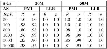
In this experiment, we compare the word pairs asso-ciation rankings obtained using PMI and LLR with CU and exact word pair counts. We use two kinds of measures, namely recall and Spearman’s correlation to measure the overlap in the rankings obtained by exact and CU counts. Intuitively, recall captures the number of word pairs that are found in both the sets and then Spearman’s correlation captures if the rela-tive order of these common word pairs is preserved in both the rankings. In our experimental setup, if the rankings match exactly, then we get a recall (R) of100% and a correlation (ρ) of1.

The results with respect to different sized counter (20 million (20M), 50 million (50M)) models are

shown in Table 1. If we compare the second and third column of the table using PMI and LLR for

20M counters, we get exact rankings for LLR

com-pared to PMI while comparing TopK word pairs.

The explanation for such a behavior is: since we are 3_{Even with other datasets we found that using counters}

lin-ear in the size of the stream leads to ARE close to zero∀counts.

# Cs 20M 50M

AS PMI LLR PMI LLR

TopK R ρ R ρ R ρ R ρ

50 1.0 1.0 1.0 1.0 1.0 1.0 1.0 1.0 100 .98 .94 1.0 1.0 1.0 1.0 1.0 1.0 500 .80 .98 1.0 1.0 .98 1.0 1.0 1.0 1000 .56 .99 1.0 1.0 .96 .99 1.0 1.0 5000 .35 .90 1.0 1.0 .85 .99 1.0 1.0 10000 .38 .55 1.0 1.0 .81 .95 1.0 1.0 Table 1:Evaluating the PMI and LLR rankings obtained using CM sketch with conservative update (CU) and Exact counts

not throwing away any infrequent word pairs, PMI will rank pairs with low frequency counts higher (Church and Hanks, 1989). Hence, we are evaluat-ing the PMI values for rare word pairs and we need counters linear in size of stream to get almost perfect ranking. This is also evident from the fourth column for50Mof the Table 1, where CU PMI ranking gets

close to the optimal as the number of counters ap-proaches stream size.

However, in some NLP problems, we are not in-terested in low-frequency items. In such cases, even using space less than linear in number of counters would suffice. In our extrinsic evaluations, we show that using space less than the length of the stream does not degrade the performance.

4 Extrinsic Evaluations

4.1 Data

Gigaword corpus (Graff, 2003) and a 50% portion

2005) are used to compute counts of words and word pairs. For both the corpora, we split the text into sentences, tokenize and convert into lower-case. We generate words and word pairs over a window of size

7. We use four different sized corpora: SubSet (used

for intrinsic evaluations in Section 3), Gigaword (GW), GigaWord +20% of web data (GWB20), and

GigaWord + 50% of web data (GWB50). Corpus

Statistics are shown below. We store exact counts of words in a hash table and store approximate counts of word pairs in the sketch. Hence, the stream size in our case is the total number of word pairs in a corpus.

Corpus Subset GW GWB20 GWB50

Unzipped _{.32 9.8 22.8 49}

Size (GB)

#of sentences _{2.00 56.78 191.28 462.60} (Million)

Stream Size _{.088 2.67 6.05 13.20} (Billion)

4.2 Semantic Orientation

Given a word, the task of finding the Semantic Ori-entation (SO) (Turney and Littman, 2003) of the word is to identify if the word is more likely to be used in positive or negative sense. We use a similar framework as used by the authors to infer the SO. We take the seven positive words (good, nice, excel-lent, positive, fortunate, correct, and superior) and the seven negative words (bad, nasty, poor, negative, unfortunate, wrong, and inferior) used in (Turney and Littman, 2003) work. The SO of a given word is calculated based on the strength of its association with the seven positive words, and the strength of its association with the seven negative words. We compute the SO of a word ”w” as follows:

SO-AS(W)= X

p∈P words

AS(p, w)₋ X

n∈N words

AS(n, w)

Where, Pwords and Nwords denote the seven pos-itive and negative prototype words respectively. We use PMI and LLR to compute association scores (AS). If this score is positive, we predict the word as positive. Otherwise, we predict it as negative.

We use the General Inquirer lexicon4 _{(Stone et}

al., 1966) as a benchmark to evaluate the semantic 4_{The General Inquirer lexicon is freely available athttp:}

//www.wjh.harvard.edu/˜inquirer/

orientation scores similar to (Turney and Littman, 2003) work. Words with multiple senses have multi-ple entries in the lexicon, we merge these entries for our experiment. Our test set consists of1597

posi-tive and1980negative words. Accuracy is used as

an evaluation metric and is defined as the percentage of number of correctly identified SO words.

0 500M 1B 1.5B 2B

60 65 70 75

Model Size

Accuracy

CU Exact

(a) SO PMI

0 500M 1B 1.5B 2B 55

60 65 70

Model Size

Accuracy

CU Exact

(b) SO LLR

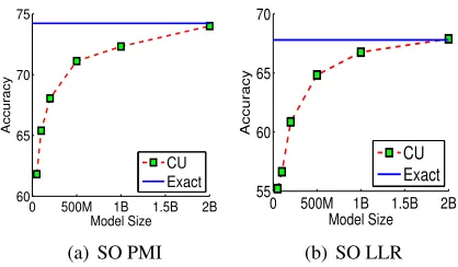
Figure 2:Evaluating Semantic Orientation using PMI and LLR with different number of counters of CU sketch built using Gi-gaword.

4.2.1 Varying sketch size

We evaluate SO of words using PMI and LLR on Gigaword (9.8GB). We compare approximate SO computed using varying sizes of CU sketches:

50million (50M),100M,200M, 500M, 1billion

(1B) and2billion (2B) counters with Exact SO. To compute these scores, we count the number of indi-vidual wordsw1andw2and the pair (w1,w2) within a window of size7. Note that computing the exact counts of all word pairs on these corpora is com-putationally expensive and memory intensive, so we consider only those pairs in which one word appears in the prototype list and the other word appears in the test set.

First, if we look at the Exact SO using PMI and LLR in Figure 2(a) and 2(b) respectively, it shows that using PMI, we get about 6 points higher

ac-curacy than LLR on this task (The 95% statistical

significance boundary for accuracy is about±1.5.).

Second, for both PMI and LLR, having more num-ber of counters improve performance.5 _{Using 2B}

counters, we get the same accuracy as Exact.

5_{We use maximum of2Bcounters (8GB main memory), as}

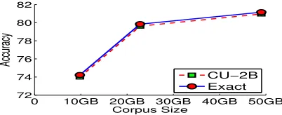
4.2.2 Effect of Increasing Corpus Size

We evaluate SO of words on three different sized corpora (see Section 4.1): GW (9.8GB), GWB20

(22.8GB), and GWB50 (49GB). First, since for this

task using PMI performs better than LLR, so we will use PMI for this experiment. Second, we will fix number of counters to 2B (CU-2B) as it performs

the best in Section 4.2.1. Third, we will compare the CU-2B counter model with the Exact over increas-ing corpus size.

We can make several observations from the Fig-ure 3: •It shows that increasing the amount of data improves the accuracy of identifying the SO of a word. We get an absolute increase of5.5points in

accuracy, when we add20%Web data to GigaWord (GW). Adding30%more Web data (GWB50), gives

a small increase of1.3points in accuracy which is

not even statistically significant. •Second, CU-2B

performs as good as exact for all corpus sizes. •

Third, the number of2B counters (bounded space)

is less than the length of stream for GWB20 (6.05B

), and GWB50 (13.2B). Hence, it shows that using

counters less than the stream length does not degrade the performance. •These results are also

compara-ble to Turney’s (2003) state-of-the-art work where they report an accuracy of82.84%. Note, they use a

billion word corpus which is larger than GWB50.

0 10GB 20GB 30GB 40GB 50GB

72 74 76 78 80 82

Corpus Size

Accuracy

CU−2B Exact

Figure 3: Evaluating Semantic Orientation of words with Ex-act and CU counts with increase in corpus size

4.3 Distributional Similarity

Distributional similarity is based on the distribu-tional hypothesis that similar terms appear in simi-lar contexts (Firth, 1968; Harris, 1954). The context vector for each term is represented by the strength of association between the term and each of the lex-ical, semantic, syntactic, and/or dependency units

that co-occur with it6_{. We use PMI and LLR to}

com-pute association score (AS) between the term and each of the context to generate the context vector. Once, we have context vectors for each of the terms, cosine similarity measure returns distributional sim-ilarity between terms.

4.3.1 Efficient Distributional Similarity

We propose an efficient approach for computing distributional similarity between word pairs using CU sketch. In the first step, we traverse the corpus and store counts of all words (except stop words) in hash table and all word pairs (except word pairs in-volving stop words) in sketch. In the second step, for a target word “x”, we consider all words (except infrequent contexts which appear less than or equal to10.) as plausible context (since it is faster than

traversing the whole corpus.), and query the sketch for vocabulary number of word pairs, and compute approximate AS between word-context pairs. We maintain only topKAS scores7 _{contexts using}

pri-ority queue for every target word “x” and save them onto the disk. In the third step, we use cosine simi-larity using these approximate topKcontext vectors to compute efficient distributional similarity.

The efficient distributional similarity using sketches has following advantages:

• It can return semantic similarity between any word pairs that are stored in the sketch.

• It can return the similarity between word pairs in time O(K).

• We do not store word pairs explicitly, and use fixed number of counters, hence the overall space required is bounded.

• The additive property of sketch (Sec. 2.1.2)

en-ables us to parallelize most of the steps in the algorithm. Thus it can be easily extended to very large amounts of text data.

We use two test sets which consist of word pairs, and their corresponding human rankings. We gen-erate the word pair rankings using efficient distri-butional similarity. We report the spearman’s rank 6_{Here, the context for a target word “x” is defined as words}

appear within a window of size7.

correlation8 _{coefficient (ρ) between the human and}

distributional similarity rankings. The two test sets are:

1. WS-353(Finkelstein et al., 2002) is a set of353

word pairs.

2. RG-65: (Rubenstein and Goodenough, 1965) is set of65word pairs.

0 500M 1B 1.5B 2B

0.1 0.15 0.2 0.25

Model Size

Accuracy

CU Exact

(a) Word Similarity PMI

0 500M 1B 1.5B 2B

0.4 0.45 0.5 0.55

Model Size

Accuracy

CU Exact

(b) Word Similarity LLR

Figure 4: Evaluating Distributional Similarity between word pairs on WS-353 test set using PMI and LLR with different number of counters of CU sketch built using Gigaword data-set.

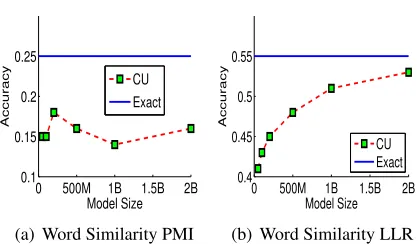
4.3.2 Varying sketch size

We evaluate efficient distributional similarity be-tween bebe-tween word pairs on WS-353 test set us-ing PMI and LLR association scores on Giga-word (9.8GB). We compare different sizes of CU

sketch (similar to SO evaluation):50million (50M),

100M, 200M, 500M, 1 billion (1B) and 2

bil-lion (2B) counters with the Exact word pair counts.

Here again, computing the exact counts of all word-context pairs on these corpora is time, and memory intensive, we generate context vectors for only those words which are present in the test set.

First, if we look at word pair ranking using exact PMI and LLR across Figures 4(a) and 4(b) respec-tively, it shows that using LLR, we get betterρ of .55compared toρof.25using PMI on this task (The 95% statistical significance boundary onρfor

WS-353 is about±.08). The explanation for such a

be-havior is: PMI rank context pairs with low frequency counts higher (Church and Hanks, 1989) compared to frequent ones which are favored by LLR. Second, 8_{To calculate the Spearman correlations values are}

trans-formed into ranks (if tied ranks exist, average of ranks is taken), and we calculate the Pearson correlation on them.

Test Set WS-353 RG-65

Model GW GW B20 GW B50 GW GW B20 GW B50

Agirre .64 .75

Exact .55 .55 .62 .65 .72 .74

CU-2B .53 .58 .62 .66 .72 .74

Table 2: Evaluating word pairs ranking with Exact and CU counts. Scores are evaluated usingρmetric.

for PMI in Fig. 4(a), having more counters does not improveρ. Third, for LLR in Fig. 4(b), having more

number of counters improve performance and using

2Bcounters, we getρclose to the Exact.

4.3.3 Effect of Increasing Corpus Size

We evaluate efficient distributional similarity be-tween word pairs using three different sized cor-pora: GW (9.8GB), GWB20 (22.8GB), and GWB50

(49GB) on two test sets: WS-353, and RG-65. First,

since for this task using LLR performs better than PMI, so we will use LLR for this experiment. Sec-ond, we will fix number of counters to 2B

(CU-2B) as it performs the best in Section 4.2.1. Third, we will compare the CU-2B counter model with the Exact over increasing corpus size. We also com-pare our results against the state-of-the-art results (Agirre) for distributional similarity (Agirre et al., 2009). We report their results of context window of size7.

We can make several observations from the Ta-ble 2: • It shows that increasing the amount of data is not substantially improving the accuracy of word pair rankings over both the test sets. • Here

again, CU-2B performs as good as exact for all cor-pus sizes.•CU-2B and Exact performs same as the state-of-the-art system. •The number of2B

coun-ters (bounded space) is less than the length of stream for GWB20 (6.05B), and GWB50 (13.2B). Hence,

here again it shows that using counters less than the stream length does not degrade the performance.

5 Dependency Parsing

de-pendency parse by linking together “most similar” words. Typically the weights on edges in the graph are parameterized as a linear function of features, with weight learned by some supervised learning al-gorithm. In this section, we ask the question: can word association scores be used to derive syntactic structures in anunsupervisedmanner?

A first pass answer is: clearly not. Metrics like PMI would assign high association scores to rare word pairs (mostly content words) leading to incor-rect parses. Metrics like LLR would assign high association scores to frequent words, also leading to incorrect parses. However, with asmall amount of linguistic side information (Druck et al., 2009; Naseem et al., 2010), we see that these issues can be overcome. In particular, we see that large data

+a little linguistics>fancy unsupervised learning

algorithms.

5.1 Graph Definition

Our approach is conceptually simple. We construct a graph over nodes in the sentence with a unique “root” node. The graph is directed and fully con-nected, and for any two words in positionsiandj,

theweightfrom wordito wordjis defined as:

wij=αascasc(wi, wj)−αdistdist(i−j) +αlingling(ti, tj)

Here, asc(wi, wj) is a association score such as

PMI or LLR computed using approximate counts from the sketch. Similarly, dist(i−j) is a simple

parameterized model of distances that favors short dependencies. We use a simple unnormalized (log) Laplacian prior of the form dist(i−j) =−|i−j−1|, centered around 1 (encouraging short links to the

right). It is negated because we need to convert dis-tances to similarities.

The final term, ling(ti, tj) asks: according to

some simple linguistic knowledge, how likely is if that the (gold standard) part of speech tag associated with word ipoints at that associated with word j?

For this, we use the same linguistic information used by (Naseem et al., 2010), which does not encode direction information. These rules are:

root_{→ {} aux, verb _}; verb_{→ {} noun,

pronoun, adverb, verb }; aux → {

verb }; noun → { adj, art, noun,

num _}; prep_{→ {} noun _}; adj _{→ {} adv

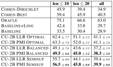
len≤10 len≤20 all

COHEN-DIRICHLET 45.9 39.4 34.9

COHEN-BEST 59.4 45.9 40.5

ORACLE 75.1 66.6 63.0

BASELINE+LING 42.4 33.8 29.7

BASELINE 33.5 30.4 28.9

CU-2B LLR OPTIMAL 62.4±7.7 51.1±3.2 41.1±1.9

CU-2B PMI OPTIMAL 63.3±7.8 52.0±3.2 41.1±2.0

CU-2B LLR BALANCED 49.1±7.6 43.6±3.3 37.2±1.9

CU-2B PMI BALANCED 49.5±8.0 45.0±3.2 38.3±2.0

CU-2B LLR SEMISUP 55.7±0.0 44.1±0.0 39.4±0.0

CU-2B PMI SEMISUP 56.5±0.0 45.8±0.0 39.9±0.0

Table 3: Comparing CU-2B build on GWB50+a little lin-guistics v/s fancy unsupervised learning algorithms.

}. We simply give an additional weight of1to any edge that agrees with one of these linguistic rules.

5.2 Parameter Setting

The remaining issue is setting the interpolation pa-rameters α associated with each of these scores.

This is a difficult problem in purely unsupervised learning. We report results on three settings. First, the OPTIMALsetting is based on grid search for op-timal parameters. This is an oracle result based on grid search over two of the three parameters (hold-ing the third fixed at 1). In our second approach,

BALANCED, we normalize the three components to “compete” equally. In particular, we scale and trans-late all three components to have zero mean and unit variance, and set theαs to all be equal to one.

Fi-nally, our third approach, SEMISUP, is based on us-ing a small amount of labeled data to set the param-eters. In particular, we use10 labeled sentences to

select parameters based on the same grid search as the OPTIMAL setting. Since this relies heavily on which10sentences are used, we repeat this

experi-ment20times and report averages.

5.3 Experiments

Our experiments are on a dependency-converted ver-sion of section 23 of the Penn Treebank using mod-ified Collins’ head finding rules. We measure accu-racies as directed, unlabeled dependency accuracy. We separately report results of sentences of length at most10, at most20and finally of all length. Note

that there is no training or cross-validation: we sim-ply run our MST parser on test data directly.

in Table 3. We compare against the following al-ternative systems. The first, Cohen-Dirichlet and Cohen-Best, are previously reported state-of-the-art results for unsupervised Bayesian dependency pars-ing (Cohen and Smith, 2010). The first is results using a simple Dirichlet prior; the second is the best reported results for any system from that paper.

Next, we compare against an “oracle” system that uses LLR extracted from the training data for the Penn Treebank, where the LLR is based on the prob-ability of observing an edge given two words. This is not a true oracle in the sense that we might be able to do better, but it is unlikely. The next two baseline system are simple right branching base-line trees. The Basebase-line system is a purely right-branching tree. The Baseline+Ling system is one that is right branchingexceptthat it can only create edges that are compatible with the linguistic rules, provided a relevant rule exists. For short sentences, this is competitive with the Dirichlet prior results.

Finally we report variants of our approach using association scores computed on the GWB50 using CU sketch with 2billion counters. We experiment

with two association scores: LLR and PMI. For each measure, we report results based on the three ap-proaches described earlier for setting the α

hyper-parameters. Error bars for our approaches are95%

confidence intervals based on bootstrap resampling. The results show that, for this task, PMI seems slightly better than LLR, across the board. The OP -TIMALperformance (based on tuning two hyperpa-rameters) is amazingly strong: clearly beating out all the baselines, and only about 15 points behind

the ORACLE system. Using the BALANCED ap-proach causes a degradation of only 3 points from

the OPTIMALon sentences of all lengths. In general, the balancing approach seems to be slightly worse than the semi-supervised approach, except on very short sentences: for those, it is substantially better. Overall, though, the results for both Balanced and Semisup are competitive with state-of-the-art unsu-pervised learning algorithms.

6 Discussion and Conclusion

The advantage of using sketch in addition to being memory and time efficient is that it contains counts for all word pairs and hence can be used to

com-pute association scores like PMI and LLR between any word pairs. We show that using sketch counts in our experiments, on the three tasks, we get perfor-mance comparable to Exact word pair counts setting and state-of-the-art system. Our method scales to49

GB of unzipped web data using bounded space of2

billion counters (8GB memory). Moreover, the

lin-earity property of the sketch makes it scalable and usable in distributed setting. Association scores and counts from sketch can be used for more NLP tasks like small-space randomized language models, word sense disambiguation, spelling correction, relation learning, paraphrasing, and machine translation. Acknowledgments

The authors gratefully acknowledge the support of NSF grant IIS-0712764 and Google Research Grant for Large-Data NLP. Thanks to Suresh Venkatasub-ramanian and Jagadeesh Jagarlamudi for useful dis-cussions and the anonymous reviewers for many helpful comments.

References

Charu C. Aggarwal and Philip S. Yu. 2010. On classi-fication of high-cardinality data streams. InSDM’10, pages 802–813.

Eneko Agirre, Enrique Alfonseca, Keith Hall, Jana Kravalova, Marius Pas¸ca, and Aitor Soroa. 2009. A study on similarity and relatedness using distributional and wordnet-based approaches. InNAACL ’09:

Pro-ceedings of HLT-NAACL.

Thorsten Brants, Ashok C. Popat, Peng Xu, Franz J. Och, and Jeffrey Dean. 2007. Large language mod-els in machine translation. InProceedings of

EMNLP-CoNLL.

Moses Charikar, Kevin Chen, and Martin Farach-Colton. 2004. Finding frequent items in data streams. Theor.

Comput. Sci., 312:3–15, January.

K. Church and P. Hanks. 1989. Word Associa-tion Norms, Mutual InformaAssocia-tion and Lexicography.

In Proceedings of ACL, pages 76–83, Vancouver,

Canada, June.

S. B. Cohen and N. A. Smith. 2010. Covariance in unsu-pervised learning of probabilistic grammars. Journal

of Machine Learning Research, 11:3017–3051.

Graham Cormode and Marios Hadjieleftheriou. 2008. Finding frequent items in data streams. InVLDB. Graham Cormode and S. Muthukrishnan. 2004. An

Gregory Druck, Gideon Mann, and Andrew McCal-lum. 2009. Semi-supervised learning of dependency parsers using generalized expectation criteria. In Pro-ceedings of the Joint Conference of the 47th Annual Meeting of the ACL and the 4th International Joint Conference on Natural Language Processing of the

AFNLP: Volume 1 - Volume 1, ACL ’09, pages 360–

368, Stroudsburg, PA, USA. Association for Compu-tational Linguistics.

Cynthia Dwork, Moni Naor, Toniann Pitassi, Guy N. Rothblum, and Sergey Yekhanin. 2010. Pan-private streaming algorithms. InIn Proceedings of ICS. Cristian Estan and George Varghese. 2002. New

di-rections in traffic measurement and accounting.

SIG-COMM Comput. Commun. Rev., 32(4).

L. Finkelstein, E. Gabrilovich, Y. Matias, E. Rivlin, Z. Solan, G. Wolfman, and E. Ruppin. 2002. Plac-ing search in context: The concept revisited. InACM

Transactions on Information Systems.

J. Firth. 1968. A synopsis of linguistic theory 1930-1955. In F. Palmer, editor, Selected Papers of J. R.

Firth. Longman.

Amit Goyal, Hal Daum´e III, and Suresh Venkatasubra-manian. 2009. Streaming for large scale NLP: Lan-guage modeling. InNAACL.

Amit Goyal, Jagadeesh Jagarlamudi, Hal Daum´e III, and Suresh Venkatasubramanian. 2010a. Sketch tech-niques for scaling distributional similarity to the web.

InGEMS workshop at ACL, Uppsala, Sweden.

Amit Goyal, Jagadeesh Jagarlamudi, Hal Daum´e III, and Suresh Venkatasubramanian. 2010b. Sketching tech-niques for Large Scale NLP. In6th WAC Workshop at

NAACL-HLT.

D. Graff. 2003. English Gigaword. Linguistic Data Con-sortium, Philadelphia, PA, January.

Z. Harris. 1954. Distributional structure. Word 10 (23), pages 146–162.

Abby Levenberg and Miles Osborne. 2009. Stream-based randomised language models for SMT. In

EMNLP, August.

Abby Levenberg, Chris Callison-Burch, and Miles Os-borne. 2010. Stream-based translation models for statistical machine translation. In Human Language Technologies: The 2010 Annual Conference of the North American Chapter of the Association for

Com-putational Linguistics, HLT ’10, pages 394–402.

As-sociation for Computational Linguistics.

Ping Li, Kenneth Ward Church, and Trevor Hastie. 2008. One sketch for all: Theory and application of condi-tional random sampling. InNeural Information

Pro-cessing Systems, pages 953–960.

G. S. Manku and R. Motwani. 2002. Approximate fre-quency counts over data streams. InVLDB.

Ryan McDonald, Fernando Pereira, Kiril Ribarov, and Jan Hajiˇc. 2005. Non-projective dependency parsing using spanning tree algorithms. InProceedings of the conference on Human Language Technology and

Em-pirical Methods in Natural Language Processing, HLT

’05, pages 523–530, Stroudsburg, PA, USA. Associa-tion for ComputaAssocia-tional Linguistics.

S. Muthukrishnan. 2005. Data streams: Algorithms and applications. Foundations and Trends in Theoretical

Computer Science, 1(2).

Tahira Naseem, Harr Chen, Regina Barzilay, and Mark Johnson. 2010. Using universal linguistic knowl-edge to guide grammar induction. InProceedings of the 2010 Conference on Empirical Methods in Natural

Language Processing, EMNLP ’10, pages 1234–1244.

Association for Computational Linguistics.

Patrick Pantel, Eric Crestan, Arkady Borkovsky, Ana-Maria Popescu, and Vishnu Vyas. 2009. Web-scale distributional similarity and entity set expansion. In

Proceedings of EMNLP.

Deepak Ravichandran, Patrick Pantel, and Eduard Hovy. 2005. Randomized algorithms and nlp: using locality sensitive hash function for high speed noun clustering.

InProceedings of ACL.

H. Rubenstein and J.B. Goodenough. 1965. Contextual correlates of synonymy. Computational Linguistics, 8:627–633.

Florin Rusu and Alin Dobra. 2007. Statistical analysis of sketch estimators. InSIGMOD ’07. ACM.

Stuart Schechter, Cormac Herley, and Michael Mitzen-macher. 2010. Popularity is everything: a new approach to protecting passwords from statistical-guessing attacks. In Proceedings of the 5th USENIX

conference on Hot topics in security, HotSec’10, pages

1–8, Berkeley, CA, USA. USENIX Association. Qinfeng Shi, James Petterson, Gideon Dror, John

Lang-ford, Alex Smola, and S.V.N. Vishwanathan. 2009. Hash kernels for structured data.J. Mach. Learn. Res., 10:2615–2637, December.

Philip J. Stone, Dexter C. Dunphy, Marshall S. Smith, and Daniel M. Ogilvie. 1966. The General Inquirer:

A Computer Approach to Content Analysis. MIT

Press.

Peter D. Turney and Michael L. Littman. 2003. Measur-ing praise and criticism: Inference of semantic orienta-tion from associaorienta-tion. ACM Trans. Inf. Syst., 21:315– 346, October.

Peter D. Turney. 2008. A uniform approach to analogies, synonyms, antonyms, and associations. In

Proceed-ings of COLING 2008.

Benjamin Van Durme and Ashwin Lall. 2009a. Prob-abilistic counting with randomized storage. In IJ-CAI’09: Proceedings of the 21st international jont

Benjamin Van Durme and Ashwin Lall. 2009b. Stream-ing pointwise mutual information. In Advances in

Neural Information Processing Systems 22.

Benjamin Van Durme and Ashwin Lall. 2010. Online generation of locality sensitive hash signatures. In