Cross Task Knowledge Constrained Self Training

Cross-Task Knowledge-Constrained Self Training

Hal Daum´e III

School of Computing University of Utah Salt Lake City, UT 84112

[email protected]

Abstract

We present an algorithmic framework for learning multiple related tasks. Our frame-work exploits a form of prior knowledge that relates the output spaces of these tasks. We present PAC learning results that analyze the conditions under which such learning is pos-sible. We present results on learning a shal-low parser and named-entity recognition sys-tem that exploits our framework, showing con-sistent improvements over baseline methods.

1 Introduction

When two NLP systems are run on the same data, we expect certain constraints to hold between their out-puts. This is a form of prior knowledge. We propose a self-training framework that uses such information to significantly boost the performance of one of the systems. The key idea is to perform self-training onlyon outputs that obey the constraints.

Our motivating example in this paper is the task pair: named entity recognition (NER) and shallow parsing (aka syntactic chunking). Consider a hid-den sentence with known POS and syntactic struc-ture below. Further consider four potential NER se-quences for this sentence.

POS:NNP NNP VBD TO NNP NN Chunk:[- NP -][- VP -][-PP-][- NP -][-NP-]

NER1:[- Per -][- O -][-Org-][- 0 -] NER2:[- Per -][- O -][- O -][- O -][- O -] NER3:[- Per -][- O -][- O -][- Org -] NER4:[- Per -][- O -][- O -][-Org-][- O -] Without ever seeing the actual sentence, can we guess which NER sequence is correct? NER1 seems

wrong because we feel like named entities should not be part of verb phrases. NER2 seems wrong be-cause there is an NNP1(proper noun) that is not part of a named entity (word 5). NER3 is amiss because we feel it is unlikely that asinglename should span more than one NP (last two words). NER4 has none of these problems and seems quite reasonable. In fact, for the hidden sentence, NER4 is correct2.

The remainder of this paper deals with the prob-lem of formulating such prior knowledge into a workable system. There are similarities between our proposed model and both self-training and co-training; background is given in Section 2. We present a formal model for our approach and per-form a simple, yet inper-formative, analysis (Section 3). This analysis allows us to define what good and bad constraints are. Throughout, we use a running example of NER using hidden Markov models to show the efficacy of the method and the relation-ship between the theory and the implementation. Fi-nally, we present full-blown results on seven dif-ferent NER data sets (one from CoNLL, six from ACE), comparing our method to several competi-tive baselines (Section 4). We see that for many of these data sets, less than one hundred labeled NER sentences are required to get state-of-the-art perfor-mance, using a discriminative sequence labeling al-gorithm (Daum´e III and Marcu, 2005).

2 Background

Self-training works by learning a model on a small amount of labeled data. This model is then

evalu-1

When we refer toNNP, we also includeNNPS.

2

The sentence is: “George Bush spoke to Congress today”

ated on a large amount of unlabeled data. Its predic-tions are assumed to be correct, and it is retrained on the unlabeled data according to its own predic-tions. Although there is little theoretical support for self-training, it is relatively popular in the natu-ral language processing community. Its success sto-ries range from parsing (McClosky et al., 2006) to machine translation (Ueffing, 2006). In some cases, self-training takes into accountmodel confidence.

Co-training (Yarowsky, 1995; Blum and Mitchell, 1998) is related to self-training, in that an algorithm is trained on its own predictions. Where it differs is that co-training learns twoseparatemodels (which are typically assumed to be independent; for in-stance by training with disjoint feature sets). These models are both applied to a large repository of un-labeled data. Examples on which these two mod-els agree are extracted and treated as labeled for a new round of training. In practice, one often also uses a notion of model confidence and only extracts agreed-upon examples for which both models are confident. The original, and simplest analysis of co-training is due to Blum and Mitchell (1998). It does not take into account confidence (to do so requires a significantlymore detailed analysis (Dasgupta et al., 2001)), but is useful for understanding the process.

3 Model

We define a formal PAC-style (Valiant, 1994) model that we call the “hints model”3. We have an instance spaceX andtwooutput spacesY₁ andY₂. We as-sume two concept classesC₁ andC₂ for each output space respectively. LetD be a distribution overX, andf1 ∈ C1(resp.,f2∈ C2) be target functions. The goal, of course, is to use a finite sample of examples drawn fromD(and labeled—perhaps with noise— byf1andf2) to “learn”h1∈ C1andh2∈ C2, which are good approximations tof1andf2.

So far we have not made use of any notion of con-straints. Our expectation is that if we constrain h1 andh2 toagree(vis-a-vis the example in the Intro-duction), then we should need fewer labeled exam-ples to learn either. (The agreement should “shrink” the size of the corresponding hypothesis spaces.) To formalize this, letχ :Y₁ × Y₂ → {0,1}be a

con-3_{The name comes from thinking of our knowledge-based}

constraints as “hints” to a learner as to what it should do.

straint function. We say that two outputsy1 ∈ Y1 andy2 ∈ Y2 arecompatibleif χ(y1, y2) = 1. We need to assume thatχis correct:

Definition 1. We say thatχ iscorrect with respect toD, f1, f2 if wheneverxhas non-zero probability

underD, thenχ(f1(x), f2(x)) = 1.

RUNNINGEXAMPLE

In our example,Y1is the space of all POS/chunk sequences and Y2 is the space of all NER se-quences. We assume that C1 and C2 are both represented by HMMs over the appropriate state spaces. The functions we are trying to learn aref1, the “true” POS/chunk labeler and f2, the “true” NER labeler. (Note that we assume f1 ∈ C1, which is obviously not true for language.)

Our constraint functionχwill require the follow-ing for agreement: (1) any NNP must be part of a named entity; (2) any named entity must be a sub-sequence of a noun phrase. This is precisely the set of constraints discussed in the introduction.

The question is: given this additional source of knowledge (i.e., χ), has the learning problem be-come easier? That is, can we learnf2(and/orf1) us-ing significantly fewer labeled examples than if we did not haveχ? Moreover, we have assumed thatχ iscorrect, but is this enough? Intuitively, no: a func-tionχthat returns1regardless of its inputs is clearly not useful. Given this, what other constraints must be placed onχ. We address these questions in Sec-tions 3.3. However, first we define our algorithm.

3.1 One-sided Learning with Hints

We begin by considering a simplified version of the “learning with hints” problem. Suppose that all we care about is learningf2. We have a small amount of data labeled byf2(call thisD) and alargeamount of data labeled byf1(call thisDunlab–”unlab” because as far asf2 is concerned, it is unlabeled).

RUNNINGEXAMPLE

We call the following algorithm “One-Sided Learning with Hints,” since it aims only to learnf2:

1: Learnh2 directly onD

2: For each example(x, y1)∈Dunlab

3: Computey2 =h2(x)

4: Ifχ(y1, y2), add(x, y2)toD

5: Relearnh2on the (augmented)D

6: Go to (2) if desired

RUNNINGEXAMPLE

In step 1, we train an NER HMM on CoNLL. On test data, this model achieves anF-score of50.8. In step 2, we run this HMM on all the WSJ data, and extract3145compatible examples. In step 3, we retrain the HMM; theF-score rises to58.9.

3.2 Two-sided Learning with Hints

In the two-sided version, we assume that we have a small amount of data labeled byf1(call thisD1), a small amount of data labeled byf2(call thisD2) and alargeamount of unlabeled data (call thisDunlab). The algorithm we propose for learning hypotheses for both tasks is below:

1: Learnh1 onD1andh2onD2.

2: For each examplex∈Dunlab:

3: Computey1 =h1(x)andy2=h2(x)

4: Ifχ(y1, y2)add(x, y1)toD1,(x, y2)toD2

5: Relearnh1onD1 andh2onD2.

6: Go to (2) if desired

RUNNINGEXAMPLE

We use3500examples from NER and1000from WSJ. We use the remaining 18447 examples as unlabeled data. The baseline HMMs achieve F -scores of50.8and76.3, respectively. In step 2, we add7512examples to each data set. After step 3, the new models achieveF-scores of54.6and79.2, respectively. The gain for NER is lower than be-fore as it is trained against “noisy” syntactic labels.

3.3 Analysis

Our goal is to prove that one-sided learning with hints “works.” That is, if C2 is learnable from large amounts of labeled data, then it is also learn-able from small amounts of labeled data and large amounts of f1-labeled data. This is formalized in Theorem 1 (all proofs are in Appendix A). How-ever, before stating the theorem, we must define an

“initial weakly-useful predictor” (terminology from Blum and Mitchell(1998)), and the notion of noisy PAC-learning in the structured domain.

Definition 2. We say thathis aweakly-useful pre-dictor of f if for all y: PrD[h(x) =y] ≥

and PrD[f(x) =y|h(x) =y0 6=y] ≥

PrD[f(x) =y] +.

This definition simply ensures that (1) h is non-trivial: it assigns some non-zero probability to every possible output; and (2)his somewhat indicative of f. In practice, we use the hypothesis learned on the small amount of training data during step (1) of the algorithm as the weakly useful predictor.

Definition 3. We say that C isPAC-learnable with noise (in the structured setting) if there exists an algorithm with the following properties. For any c ∈ C, any distribution D overX, any 0 ≤ η ≤

1/|Y|, any 0 < < 1, any0 < δ < 1 and any η ≤ η0 < 1/|Y|, if the algorithm is given access

to examples drawn EXη_SN(c,D) and inputs, δand η0, then with probability at least 1 −δ, the

algo-rithm returns a hypothesish∈ Cwith error at most . Here, EXη_SN(c,D) is a structured noise oracle, which draws examples fromD, labels them bycand randomly replaces with another label with prob.η.

Note here the rather weak notion of noise: en-tire structures are randomly changed, rather than in-dividual labels. Furthermore, the error is 0/1 loss over the entire structure. Collins (2001) establishes learnability results for the class of hyperplane mod-els under 0/1 loss. While not stated directly in terms of PAC learnability, it is clear that his results apply. Taskar et al. (2005) establishtighterbounds for the case of Hamming loss. This suggests that the re-quirement of 0/1 loss is weaker.

As suggested before, it is not sufficient for χ to simply be correct (the constant 1 function is cor-rect, but not useful). We need it to be discriminating, made precise in the following definition.

Definition 4. We say thediscriminationofχforh0 isPrD[χ(f1(x), h0(x))]−1.

RUNNINGEXAMPLE

In the NER HMM, leth0be the HMM obtained by training on the small labeled NER data set andf1 is the true syntactic labels. We approximatePrD

by an empirical estimate over the unlabeled distri-bution. This gives a discrimination is41.6for the constraint function defined previously. However, if we compare against “weaker” constraint functions, we see the appropriate trend. The value for the con-straint based only on POS tags is39.1(worse) and for the NP constraint alone is27.0(much worse).

Theorem 1. Suppose C2 is PAC-learnable with

noise in the structured setting, h0₂ is a weakly use-ful predictor off2, andχis correct with respect to

D, f1, f2, h02, and has discrimination≥2(|Y| −1).

ThenC2is also PAC-learnable with one-sided hints.

The way to interpret this theorem is that it tells us that if the initialh2we learn in step 1 of the one-sided algorithm is “good enough” (in the sense that it is weakly-useful), then we can use it as specified by the remainder of the one-sided algorithm to obtain an arbitrarily goodh2 (via iterating).

The dependence on |Y| is the discrimination bound forχis unpleasant for structured problems. If we wish to findM unlabeled examples that satisfy the hints, we’ll need a total of at least2M(|Y| −1) total. This dependence can be improved as follows. Suppose that our structure is represented by a graph over verticesV, each of which can take a label from a setY. Then,|Y| =YV

, and our result requires thatχbe discriminating on an order exponential in V. Under the assumption that χ decomposes over the graph structure (true for our example) and that C2is PAC-learnable with per-vertex noise, then the discrimination requirement drops to2|V|(|Y| −1).

RUNNINGEXAMPLE

In NER, |Y| = 9 and |V| ≈ 26. This means that the values from the previous example look not quite so bad. In the 0/1 loss case, they are com-pared to1025_{; in the Hamming case, they are} com-pared to only416. The ability of the one-sided al-gorithm follows the same trends as the discrimi-nation values. Recall the baseline performance is

50.8. With both constraints (and a discrimination value of41.6), we obtain a score of58.9. With just the POS constraint (discrimination of39.1), we ob-tain a score of 58.1. With just the NP constraint (discrimination of27.0, we obtain a score of54.5.

The final question is how one-sided learning re-lates to two-sided learning. The following definition and easy corollary shows that they are related in the obvious manner, but depends on a notion of uncor-relation betweenh0₁andh0₂.

Definition 5. We say that h1 and h2 are un-correlated if PrD[h1(x) =y1|h2(x) =y2, x] =

PrD[h1(x) =y1|x].

Corollary 1. Suppose C1 and C2 are both

PAC-learnable in the structured setting, h0₁ and h0₂ are weakly useful predictors of f1 and f2, and χ is

correct with respect to D, f1, f2, h01 and h02, and

has discrimination≥ 4(|Y| −1)2 (for 0/1 loss) or

≥4|V|2(|Y| −1)2(for Hamming loss), and thath0₁ andh0₂ are uncorrelated. ThenC1 andC2 are also

PAC-learnable with two-sided hints.

Unfortunately, Corollary 1 dependsquadratically on the discrimination term, unlike Theorem 1.

4 Experiments

In this section, we describe our experimental results. We have already discussed some of them in the con-text of the running example. In Section 4.1, we briefly describe the data sets we use. A full descrip-tion of the HMM implementadescrip-tion and its results are in Section 4.2. Finally, in Section 4.3, we present results based on a competitive, discriminatively-learned sequence labeling algorithm. All results for NER and chunking are in terms of F-score; all re-sults for POS tagging are accuracy.

4.1 Data Sets

4.2 HMM Results

The experiments discussed in the preceding sections are based on a generative hidden Markov model for both the NER and syntactic chunking/POS tagging tasks. The HMMs constructed use first-order tran-sitions and emissions. The emission vocabulary is pruned so that any word that appears≤1time in the training data is replaced by a unique *unknown*

token. The transition and emission probabilities are smoothed with Dirichlet smoothing,α= 0.001(this was not-aggressively tuned by hand on one setting). The HMMs are implemented as finite state models in the Carmel toolkit (Graehl and Knight, 2002).

The various compatibility functions are also im-plemented as finite state models. We implement them as a transducerfromPOS/chunk labelstoNER labels (though through the reverse operation, they can obviously be run in the opposite direction). The construction is with a single state with transitions:

• (NNP,?)maps toB-*andI-*

• (?,B-NP)maps toB-*andO

• (?,I-NP)maps toB-*,I-*andO

• Single exception:(NNP,x), wherexisnotan NP tag maps to anything (this is simply to avoid empty composition problems). This occurs in 100of the212kwords in the Treebank data and more rarely in the automatically tagged data.

4.3 One-sided Discriminative Learning

In this section, we describe the results of one-sided discriminative labeling with hints. We use the true syntactic labels from the Penn Treebank to derive the constraints (this is roughly9000sentences). We use the LaSO sequence labeling software (Daum´e III and Marcu, 2005), with its built-in feature set.

Our goal is to analyze two things: (1) what is the effect of the amount of labeled NER data? (2) what is the effect of the amount of labeled syntactic data from which the hints are constructed?

To answer the first question, we keep the amount of syntactic data fixed (at 8936 sentences) and vary the amount of NER data in N ∈ {100,200,400,800,1600}. We compare models with and without the default gazetteer information from the LaSO software. We have the following models for comparison:

• A default “Baseline” in which we simply train the NER model without using syntax.

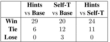
Hints Self-T Hints

vsBase vsBase vsSelf-T

Win 29 20 24

Tie 6 12 11

Lose 0 3 0

Table 1: Comparison between hints, self-training and the (best) baseline for varying amount of labeled data.

• In “POS-feature”, we do the same thing, but we first label the NER data using a tagger/chunker trained on the8936syntactic sentences. These labels are used as features for the baseline.

• A “Self-training” setting where we use the 8936syntactic sentences as “unlabeled,” label them with our model, and then train on the results. (This is equivalent to a hints model where χ(·,·) = 1 is the constant 1 func-tion.) We use model confidence as in Blum and Mitchell (1998).4

The results are shown in Figure 1. The trends we see are the following:

• More data always helps.

• Self-training usually helps over the baseline (though not always: for instance in wl and parts of cts and bn).

• Adding the gazetteers help.

• Adding the syntactic features helps.

• Learning with hints, especially for ≤ 1000 training data points, helps significantly, even over self-training.

We further compare the algorithms by looking at how many training setting has each as the winner. In particular, we compare both hints and self-training to the two baselines, and then compare hints to self-training. If results are not significant at the 95% level (according to McNemar’s test), we call it a tie. The results are in Table 1.

In our second set of experiments, we consider the role of the syntactic data. For this experiment, we hold the number of NER labeled sentences constant (atN = 200) and vary the amount of syntactic data inM ∈ {500,1000,2000,4000,8936}. The results of these experiments are in Figure 2. The trends are:

• The POS feature is relatively insensitive to the amount of syntactic data—this is most likely because it’s weight is discriminatively adjusted

4

0 1000 2000 0.2

0.3 0.4 0.5 0.6 0.7

wl

0 1000 2000 0.4

0.5 0.6 0.7 0.8

nw

0 1000 2000 0.4

0.5 0.6 0.7 0.8 0.9

conll

0 1000 2000 0.4

0.5 0.6 0.7 0.8

bc

0 1000 2000 0.2

0.3 0.4 0.5 0.6 0.7

un

0 1000 2000 0.75

0.8 0.85 0.9 0.95

cts

0 1000 2000 0

0.2 0.4 0.6 0.8

bn

POS−feature Hints (no gaz) Baseline (no gaz) Hints (w/ gaz) Baseline (w/ gaz) Self−train (no gaz) Self−train (w/ gaz)

Figure 1: Results of varying the amount of NER labeled data, for a fixed amount (M = 8936) of syntactic data.

Hints Self-T Hints

vsBase vsBase vsSelf-T

Win 34 28 15

Tie 1 7 20

Lose 0 0 0

Table 2: Comparison between hints, self-training and the (best) baseline for varying amount of unlabeled data.

by LaSO so that if the syntactic information is bad, it is relatively ignored.

• Self-training performance oftendegradesas the amount of syntactic data increases.

• The performance of learning with hints in-creases steadily with more syntactic data.

As before, we compare performance between the different models, declaring a “tie” if the difference is not statistically significant at the 95% level. The results are in Table 2.

In experiments not reported here to save space, we experimented with several additional settings. In one, we weight the unlabeled data in various ways: (1) to make it equal-weight to the labeled data; (2) at10%weight; (3) according to the score produced by the first round of labeling. None of these had a

significant impact on scores; in a few cases perfor-mance went up by1, in a few cases, performance went down about the same amount.

4.4 Two-sided Discriminative Learning

In this section, we explore the use of two-sided discriminative learning to boost the performance of our syntactic chunking, part of speech tagging, and named-entity recognition software. We continue to use LaSO (Daum´e III and Marcu, 2005) as the se-quence labeling technique.

The results we present are based on attempting to improve the performance of a state-of-the-art system train onallof the training data. (This is in contrast to the results in Section 4.3, in which the effect of us-ing limited amounts of data was explored.) For the POS tagging and syntactic chunking, we being with all8936sentences of training data from CoNLL. For the named entity recognition, we limit our presenta-tion to results from the CoNLL 2003 NER shared task. For this data, we have roughly14ksentences of training data, all of which are used. In both cases, we reserve10%as development data. The develop-ment data is use to do early stopping in LaSO.

En-0 5000 10000 0.35

0.4 0.45 0.5 0.55 0.6 0.65

wl

0 5000 10000 0.55

0.6 0.65 0.7 0.75 0.8

nw

0 5000 10000 0.5

0.6 0.7 0.8 0.9

conll

0 5000 10000 0.5

0.6 0.7 0.8 0.9

bc

0 5000 10000 0.2

0.3 0.4 0.5 0.6 0.7

un

0 5000 10000 0.75

0.8 0.85 0.9 0.95

cts

0 5000 10000 0.2

0.4 0.6 0.8 1

bn

POS−feature Hints (no gaz) Baseline (no gaz)

Hints (w/ gaz) Baseline (w/ gaz) Self−train (no gaz) Self−train (w/ gaz)

Figure 2: Results of varying amount of syntactic data for a fixed amount of NER data (N = 200sentences).

glish (previously used for self-training of parsers (McClosky et al., 2006)). These1msentences were selected by dev-set relativization against the union of the two development data sets.

Following similar ideas to those presented by Blum and Mitchell (1998), we employ two slight modifications to the algorithm presented in Sec-tion 3.2. First, in step (2b) instead of adding all allowable instances to the labeled data set, we only add the topR(for some hyper-parameterR), where “top” is determined by average model confidence for the two tasks. Second, Instead of using thefull un-labeled set to label at each iteration, we begin with a random subset of10Runlabeled examples and an-other add random10Revery iteration.

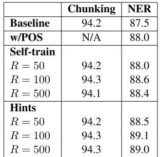
We use the same baseline systems as in one-sided learning: a Baseline that learns the two tasks inde-pendently; a variant of the Baseline on which the output of the POS/chunker is used as a feature for the NER; a variant based on self-training; the hints-based method. In all cases, wedouse gazetteers. We run the hints-based model for10iterations. For self-training, we use10Runlabeled examples (so that it had access to the same amount of unlabeled data as the hints-based learning after all10 iterations). We used three values ofR: 50,100,500. We select the

Chunking NER Baseline 94.2 87.5

w/POS N/A 88.0

Self-train

R= 50 94.2 88.0

R= 100 94.3 88.6 R= 500 94.1 88.4

Hints

R= 50 94.2 88.5

R= 100 94.3 89.1 R= 500 94.3 89.0

Table 3: Results on two-sided learning with hints.

best-performing model (by the dev data) over these ten iterations. The results are in Table 3.

enormous, but are significant (at the 95% level, as measured by McNemar’s test). Unfortunately, the improvements for learning with hints over the self-training model are only significant at the 90% level.

5 Discussion

We have presented a method for simultaneously learning two tasks using prior knowledge about the relationship between their outputs. This is related to joint inference (Daum´e III et al., 2006). How-ever, we do not require that that a single data set be labeled for multiple tasks. In all our examples, we use separate data sets for shallow parsing as for named-entity recognition. Although all our exper-iments used the LaSO framework for sequence la-beling, there is notingin our method that assumes any particular learner; alternatives include: condi-tional random fields (Lafferty et al., 2001), indepen-dent predictors (Punyakanok and Roth, 2001), max-margin Markov networks (Taskar et al., 2005), etc.

Our approach, both algorithmically and theoreti-cally, is most related to ideas in co-training (Blum and Mitchell, 1998). The key difference is that in co-training, one assumes that the two “views” are on the inputs; here, we can think of the two out-put spaces as being the difference “views” and the compatibility functionχbeing a method for recon-ciling these two views. Like the pioneering work of Blum and Mitchell, the algorithm we employ in practice makes use of incrementally augmenting the unlabeled data and using model confidence. Also like that work, we do not currently have a theoret-ical framework for this (more complex) model.5 It would also be interesting to exploresofthints, where the range ofχis[0,1]rather than{0,1}.

Recently, Ganchev et al. (2008) proposed a co-regularization framework for learning across multi-ple related tasks with different output spaces. Their approach hinges on a constrained EM framework and addresses a quite similar problem to that ad-dressed by this paper. Chang et al. (2008) also propose a “semisupervised” learning approach quite similar to our own model. The show very promis-ing results in the context of semantic role labelpromis-ing.

5

Dasgupta et al. (2001) proved, three years later, that a for-mal model roughly equivalent to the actual Blum and Mitchell algorithmdoeshave solid theoretical foundations.

Given the apparent (very!) recent interest in this problem, it would be ideal to directly compare the different approaches.

In addition to an analysis of the theoretical prop-erties of the algorithm presented, the most com-pelling avenue for future work is to apply this frame-work to other task pairs. With a little thought, one can imagine formulating compatibility functions be-tween tasks like discourse parsing and summariza-tion (Marcu, 2000), parsing and word alignment, or summarization and information extraction.

Acknowledgments

Many thanks to three anonymous reviewers of this papers whose suggestions greatly improved the work and the presentation. This work was partially funded by NSF grant IIS 0712764.

A Proofs

The proof of Theorem 1 closes follows that of Blum and Mitchell (1998).

Proof (Theorem 1, sketch). Use the following nota-tion: ck = PrD[h(x) = k], pl = PrD[f(x) = l],

q_l|k = PrD[f(x) = l|h(x) = k]. Denote by A

the set of outputs that satisfy the constraints. We are interested in the probability thath(x)is erroneous, given thath(x)satisfies the constraints:

p(h(x)∈ A\{l} |f(x) =l)

= X

k∈A\{l}

p(h(x) =k|f(x) =l) = X

k∈A\{l}

ckql|k/pl

≤X

k∈A

ck(|Y| −1 +

X

l6=k

1/pl)≤2

X

k∈A

ck(|Y| −1)

Here, the second step is Bayes’ rule plus definitions, the third step is by the weak initial hypothesis as-sumption, and the last step is by algebra. Thus, in order to get a probability of error at mostη, we need P

k∈Ack= Pr[h(x)∈ A]≤η/(2(|Y| −1)).

The proof of Corollary 1 is straightforward.

References

Avrim Blum and Tom Mitchell. 1998. Combining la-beled and unlala-beled data with co-training. In Pro-ceedings of the Conference on Computational Learn-ing Theory (COLT), pages 92–100.

Ming-Wei Chang, Lev Ratinov, Nicholas Rizzolo, and Dan Roth. 2008. Learning and inference with con-straints. In Proceedings of the National Conference on Artificial Intelligence (AAAI).

Michael Collins. 2001. Parameter estimation for statistical parsing models: Theory and practice of distribution-free methods. InInternational Workshop on Parsing Technologies (IWPT).

Sanjoy Dasgupta, Michael Littman, and David McAllester. 2001. PAC generalization bounds for co-training. In Advances in Neural Information Processing Systems (NIPS).

Hal Daum´e III and Daniel Marcu. 2005. Learning as search optimization: Approximate large margin meth-ods for structured prediction. InProceedings of the In-ternational Conference on Machine Learning (ICML). Hal Daum´e III, Andrew McCallum, Ryan McDonald, Fernando Pereira, and Charles Sutton, editors. 2006.

Workshop on Computationally Hard Problems and Joint Inference in Speech and Language Process-ing. Proceedings of the Conference of the North American Chapter of the Association for Computa-tional Linguistics and Human Language Technology (NAACL/HLT).

Kuzman Ganchev, Joao Graca, John Blitzer, and Ben Taskar. 2008. Multi-view learning over structured and non-identical outputs. InProceedings of the Conver-ence on Uncertainty in Artificial IntelligConver-ence (UAI). Jonathan Graehl and Kevin Knight. 2002. Carmel

fi-nite state transducer package. http://www.isi. edu/licensed-sw/carmel/.

John Lafferty, Andrew McCallum, and Fernando Pereira. 2001. Conditional random fields: Probabilistic mod-els for segmenting and labeling sequence data. In Pro-ceedings of the International Conference on Machine Learning (ICML).

Daniel Marcu. 2000. The Theory and Practice of Dis-course Parsing and Summarization. The MIT Press, Cambridge, Massachusetts.

Mitch Marcus, Mary Ann Marcinkiewicz, and Beatrice Santorini. 1993. Building a large annotated corpus of English: The Penn Treebank. Computational Linguis-tics, 19(2):313–330.

David McClosky, Eugene Charniak, and Mark Johnson. 2006. Effective self-training for parsing. In Proceed-ings of the Conference of the North American Chapter of the Association for Computational Linguistics and Human Language Technology (NAACL/HLT).

Vasin Punyakanok and Dan Roth. 2001. The use of clas-sifiers in sequential inference. InAdvances in Neural Information Processing Systems (NIPS).

Lance A. Ramshaw and Mitchell P. Marcus. 1995. Text chunking using transformation-based learning. In Pro-ceedings of the Third ACL Workshop on Very Large Corpora.

Ben Taskar, Vassil Chatalbashev, Daphne Koller, and Carlos Guestrin. 2005. Learning structured predic-tion models: A large margin approach. InProceedings of the International Conference on Machine Learning (ICML), pages 897–904.

Erik F. Tjong Kim Sang and Sabine Buchholz. 2000. Introduction to the CoNLL-2000 shared task: Chunk-ing. InProceedings of the Conference on Natural Lan-guage Learning (CoNLL).

Erik F. Tjong Kim Sang and Fien De Meulder. 2003. In-troduction to the CoNLL-2003 shared task: Language-independent named entity recognition. InProceedings of Conference on Computational Natural Language Learning, pages 142–147.

Nicola Ueffing. 2006. Self-training for machine trans-lation. In NIPS workshop on Machine Learning for Multilingual Information Access.

Leslie G. Valiant. 1994. A theory of the learnable. An-nual ACM Symposium on Theory of Computing, pages 436–445.

Ralph Weischedel, editor. 2004. Automatic Content Ex-traction Workshop (ACE-2004), Alexandria, Virginia, September 20–22.