Abstract—This paper studies the optimal collision avoidance strategies in a close proximity coplanar cooperative encounter between two participants with unequal turn capabilities. The synthesis of optimal control is presented in the form of 2D diagram with dispersal curves partitioning the plane of the initial relative positions into sub-regions of initial positions for different optimal strategies. To resolve the non-uniqueness of the optimal strategies associated with the dispersal curves, we introduce the maneuver time as an additional performance criterion. We show that while the optimal strategies that start at the dispersal point often have identical maneuver time for a classical problem of collision avoidance of identical participants, this is no longer the case when the participants have unequal turn capabilities. We show that a unique strategy with smaller maneuver time can be identified based on the non-dimensional parameter of the problem. Efficient numerical algorithms for calculation of the maneuver time for optimal strategies are also presented. The results in this paper are applicable in aviation, ship collision avoidance and robotics.
Index Terms — Close proximity, Collision avoidance, Cooperative maneuvers, Dispersal curves, Mayer problem, Maneuver time, Optimal control, Pontryagin maximum principle, Unequal turn rates.
I. INTRODUCTION
Close proximity encounters (i.e., where the participants are sufficiently close in space and time to be of operational concern) can occur in many applications in aviation, navigation and robotics. For such situations, the maximization of terminal miss distance (which is a minimal distance between the participants during the maneuver) is an adequate and important objective [1]-[5]. The coplanar close proximity encounter between two aircraft (ships) was first studied by Merz [1], [2] (and a rigorous analysis is given in [3]) who presented the synthesis of the optimal control for identical aircraft (ships) in the form of 2D diagram. The Merz solution partitions the plane of the initial relative positions of the aircraft into two half-planes. In one half-plane, the relative distance is decreasing (converging). For the other half-plane, divergence (increase in relative distance) occurs. The
Manuscript received March 5, 2010.
T. Tarnopolskaya is with the Commonwealth Scientific and Industrial Research Organisation (CSIRO), Mathematics, Informatics and Statistics, Locked Bag 17, North Ryde, NSW 1670, Australia (phone: +61 2 9325 3254; fax+61 2 9325 3200; e-mail: [email protected]).
N. L. Fulton is with the Commonwealth Scientific and Industrial Research Organisation (CSIRO), Mathematics, Informatics and Statistics,
convergence half-plane is further partitioned into the three sub-regions corresponding to the initial relative positions for different optimal strategies. Such diagram establishes the optimal collision avoidance strategy for both participants based on their initial relative position and orientation and presents an important tool for setting and validating the traffic rules. Recently, earlier analyses have been extended to the case of participants with unequal turn capabilities [4], [5]. It has been shown that the case of identical participants studied by Merz presents a degenerate case of this more general situation.
This paper continues the study in [4], [5] and focuses on the dispersal curves for the case of participants with unequal turn rates. Dispersal curve (which is a planar case of dispersal or singular surface in differential games theory [6]) separates the regions of different optimal strategies. Such curve presents a locus of the initial positions for which optimal solution is not unique (i.e. there are two optimal strategies that result in the same terminal miss distance). Dispersal curve therefore involves conflicting decisions by the participants as to which of two equally optimal paths to take. In the case of coplanar close proximity encounter, there is also a triple point present, where the three optimal strategies result in the same terminal miss distance. This paper introduces an additional performance criterion that can be used to select a unique optimal strategy that originates at a dispersal point or the triple point. Such a criterion is the maneuver time. This criterion is not only important in a theoretical sense as a measure of efficiency but also in a practical sense as an input to the flight management system / autopilot system design.
The analysis in this paper is based on the Pontryagin maximum principle for a Mayer problem. Main results of the paper can be summarized as follows. We show that while for the case of identical participants the maneuver time of two optimal strategies originated at the dispersal point is often identical, this is not the case for participants with unequal turn capabilities. We show that a unique strategy for non-identical participants can be selected if the maneuver time is considered as an additional performance criterion. A simple analytic characterisation of the unique strategy with smaller maneuver time is established. Efficient numerical algorithms for calculation of the maneuver time are also presented. Due to the page limit, only the RR-LL dispersal curve and the triple point are considered, but it is straightforward to extend the analysis to the other dispersal curves.
Dispersal Curves for Optimal Collision
Avoidance in a Close Proximity Encounter: a
Case of Participants with Unequal Turn Rates
II. OPTIMIZATION PROBLEM
As common for close proximity encounter models [1]-[5], the underlying assumption is that the linear speeds of the participants are constant. The maximization of the terminal miss distance is adopted as a performance criterion.
The nondimensional equations of motion of two participants with equal linear speeds but unequal turn capabilities in the moving polar coordinate system are [1]-[5]
1
1 2
cos cos( )
[sin sin( )] /r f( , ),u (1)
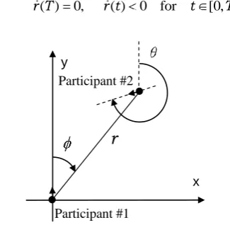
where T ( , , )r ; r, , specify the non-dimensional instantaneous relative distance between the participants and the instantaneous angles defining the relative direction of their motion (see Fig. 1), r: r R/ 1min, R1min is the lower bound on the turn radius of the first participant; 1, 2are the non-dimensional angular speeds of the participants scaled so that they are contained in the interval [-1, 1], with positive values corresponding to the right turns (from the point of view of the participant), and negative values corresponding to the left turn, 1 1/ 1max, 2 2/ 2max, where 1, 2are the angular speeds, 1max, 2max are the physical bounds on the angular speeds of the participants; is the nondimensional parameter of the problem,
max max
2 / 1 0. The derivatives with respect to the non-dimensional time t t( : t 1max )are denoted with dots. The domains for the variables , are defined as
, 0 2 .
The system of ordinary differential equations (1) can be viewed as a control system with the state vector
( , , )
T r and control function
1 2 ( , ), T
u
2
: [0, ] ; , [ 1,1] [ 1,1].
u T U U R U
The non-dimensional maneuver time T (also known as the terminal time) is defined as the time to closest approach between the participants. It is defined by the conditions
( ) 0,
r T r t( ) 0 for t [0, ].T (2)
The objective is to maximize the terminal miss distance ( , )u rt T rT over all admissible controls. Thus, the performance index is a function of the terminal time only. As the terminal time T is unknown, the problem can be considered as a Mayer problem with free terminal point.
It is easy to see that the first equation of (1) together with the first of conditions (2) yield two possible terminal conditions:
1. T 0; (3) 2. T T/2 , T T/2. (4)
III. NECESSARY CONDITIONS FOR OPTIMALITY The Hamiltonian function in the polar coordinate system is given by:
1 2
1
( , , ) ( , )
[ cos cos( )] ( )
{ [sin sin( )] / },
T
r
H u f u
r
(5)
where the adjoint variables T ( r, , ) satisfy the equations H, that is
2 [sin sin( )] /
(sin sin( )) [cos cos( )] /
sin( ) cos( ) /
r
r
r
r r
(6)
with boundary conditions ( )T ( ( ), )T u [1, 0, 0]T. Using the Pontryagin Maximum Principle [7], it can be shown ([3], [4]) that the terminal conditions (3) and (4) yield two types of possible optimal strategies: 1) terminal condition (3) corresponds to 1 2 1 (the participants are turning with maximum possible angular speed in opposite directional sense). We will call such strategies right-left (RL) and left-right (LR) strategies, where the first letter indicates the strategy of the first participant (located in the origin of Fig.1); 2) terminal condition (4) results in 1 2 1 (both participants are turning with the maximum possible angular speed in the same directional sense). Such strategies will be called right-right (RR) and left-left (LL) strategies.
Using the transformation of variables 2 2
y x
r , ,
sin x
r rcos y, (1) can be re-written in the Cartesian coordinates and presented in terms of backward (retrograde) derivatives as
1 sin , 1 1 cos , 1 2,
x y y x (7) where circles denote the derivative with respect to
( T t).
Solving (7) subject to the boundary conditions 0 T,
x x
0 T,
y y and one of the two terminal conditions (3), (4) yields the following two cases:
Case I. T 0, 1 2 1. This case corresponds to
[image:2.595.80.243.558.717.2]the RL and LR strategies. The solution of (7) is given by Figure 1: Schematics of the coplanar
encounter in the moving coordinate system
r
x y
1 1
1 1
1 1
1
(1 ) for 1,
2 (1 ) for 1,
sin( ) [1 cos[(1 ) ] /
(1 ) cos / ],
cos( ) (1 ) sin /
sin[(1 ) ] / ,
T T
T T
x r
y r
(8)
where subscript “T” refers to the terminal instant. For T, (8) describes the locus of the initial conditions
) ,
(
0 0 0
0 xt y yt
x and takes the form
For 1 1:
2
0 0 0
2 2
0 0 0
{ 1 cos / (1 ) cos[ / (1 )] / }
{ (1 ) sin[ / (1 )] / sin / } T,
x
y r (9)
For 1 1:
0 0
2
0 0 0
2 2 0
{ (1 ) cos[( 2 ) / (1 )] / 1
cos / } { (1 ) sin[( 2 ) / (1 )] /
sin / } T.
x
y r
(10)
Case II. T 2 T 2 or T 2 T; 1 2 1. This
case corresponds to the RR and LL strategies. The solution of (7) takes the form
1
1
1 1 1
1 1 1
1 1 1
(1 ) , cos( ) sin
{sin( ) sin[ (1 ) ]} / , sin( ) cos( ) /
(1 cos ) cos[ (1 ) ] / . T
T T
T T
T T T
T
y r
x r
(11)
For T we have 0 1(1 )T T, and the two branches of the initial conditions for the state variables
) ,
(x y are given by: For T T /2:
2 2
0 1 0 0 1 0
2
0 1
1 0 1
[ (1 cos / )] ( sin / ) 2 2 cos[ (1 ) ] /
2 (1 1/ ) sin[( (1 ) ) / 2], T
T
x y
r T
r T
(12)
For T T /2 :
2 2
0 1 0 0 1 0
2
0 1
1 0 1
[ (1 cos / )] ( sin / ) 2 2 cos[ (1 ) ] /
2 (1 1/ ) sin[( (1 ) ) / 2]. T
T
x y
r T
r T
(13)
IV. DISPERSAL CURVES AND SYNTHESIS OF OPTIMAL CONTROL
In order to select the optimal trajectories from the sets of extremals (8), (11), one should: (a) select the trajectories such that the distance between the participants decreases on the time interval t [0,T]; (b) amongst such trajectories, select those that maximize the performance criterion (the terminal miss distance). These steps are discussed in details in [4]. The synthesis of optimal control was also constructed there. Firstly, we summarize several results from [4] that are useful for the analysis in this paper.
Property 1 For 0 , possible optimal strategies are
right-right (RR), left-left (LL) and right-left (RL) strategies.
For 0 2 , possible optimal strategies are
right-right(RR), left-left (LL) and left-right (LR) strategies;
Property 2 For given rT, 0(0 0 ) and , the locus
of the initial relative positions for optimal trajectories consists of the arcs of the loci of the initial positions for the
RR strategy (13) ( 1 1), the LL strategy (12) ( 1 1) and
the RL strategy (9). A point of simultaneous intersection of
these loci is called atriple point. For rT rTtp(where rTtpis
the terminal miss distance at the triple point), the locus of the initial relative positions for optimal strategies consists of the arcs of the loci for the RR and the LL strategies (13) and (12) only. The points of intersection of these loci are called dispersal points;
Property 3 A straight line passing through the origin
with tan tan( 0/2) represents the locus rt 0 0 . It
divides the plane of the initial relative positions ( , )x y into
the two half-planes of instantaneously diverging and converging distance between the participants at the beginning of the maneuver;
Property 4 The half-plane of converging relative distance
can be further partitioned into 3 sub-regions of initial relative positions for three optimal strategies, with dispersal curves separating the sub-regions of different optimal strategies;
Property 5 Straight lines passing through the origin with
0 1 1
tan t T tan{[ (1 ) ] / 2},T 1, (14)
represent the loci rt T 0 for the RR and the LL strategies.
We call these lines the RR and LL loci of terminal relative
positions. For given 0 and , the trajectories that start on
the loci of the initial conditions for the RR or LL strategies (12), (13) end on lines (14).
The synthesis of optimal control for participants with unequal turn capabilities can be presented as a 2D diagram (similar to that first presented by Merz for identical participants) that partitions the plane of the initial relative
[image:3.595.345.500.538.745.2]
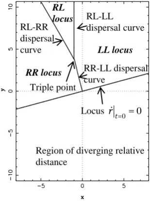
Figure 2: Synthesis of optimal control diagram, 0 5 / 6; 1.
Region of diverging relative distance
RR-LL dispersal curve
RL-LL dispersal curve RL-RR
dispersal curve
Triple point Locus
0 0 t
r
LL locus
positions into the sub-regions of different optimal strategies (Fig.2 ).
While Fig. 2 shows the synthesis of optimal control diagram for the case of identical participants, the structure of synthesis for non-identical participants is similar. The regions of initial relative positions for the RR, LL and RL optimal strategies (called RR, LL and RL loci respectively) are separated by the dispersal curves. For 0 0 , there are 3 dispersal curves: the RR-LL dispersal curve, the RL-LL and the RL-RR dispersal curves. A triple point (i.e. the point on the plane of initial relative positions such that the RR, LL and RL strategies started at this point result in the same terminal miss distance) is also illustrated in Fig. 2.
In what follows, we only consider the case 0 0 for the sake of brevity. To find the triple point, one needs to find the point of intersection of the loci of the initial relative position for the LL strategy (12), the RR strategy (13) and the locus of the initial relative positions of the RL strategy (9). Thus, one needs to satisfy the conditions
/ 2 / 2
/ 2 / 2
/ 2 / 2 ( ) ( ) , ( ) ( ) , ( ) ( , ), ( ) ( , ),
T T T T
T T T T
T T T T tp tp LL RR LL RR tp tp LL RR LL RR
tp tp tp
LL RL
LL T T
tp tp
LL TP RL
LL T T
x T x T y T y T x T x r y T y r
(15)
where TLLtp and TRRtp are the maneuver times for the LL and the RR strategies at the triple point respectively, rTtp and Ttp are the terminal miss distance and the terminal relative bearing at the triple point respectively. Conditions (15) can be reduced to the system of three trigonometric equations
0 0
0
0 0
0 0
0
0 sin(( ) / 2) 2 cos /
sin(( ) / 2) cos 2
cos [cos( ) cos( )] / , 0 cos(( ) / 2) 2sin /
cos(( ) / 2) sin
tp tp tp
LL LL
T
tp tp tp tp
RR RR LL
T
tp tp tp
RR LL RR
tp tp tp
LL LL
T
tp tp tp tp
RR RR LL
T
r T T
r T T T
T T T
r T T
r T T T
0 0 2 0 2 0 0 0 0
sin [sin( ) sin( )] / ,
( ) { sin(( ) / 2) cos 2
cos( ) / ( 1) cos( / (1 )) / }
{ cos(( ) / 2) sin 2
sin( ) / ( 1) sin[
tp tp tp
RR LL RR
tp tp tp tp tp
LL LL LL
T T
tp LL
tp tp tp tp
LL LL LL
T
tp LL
T T T
r r T T T
T
r T T T
T 2
0/ (1 )] / } , (16)
with the unknowns (TLLtp,TRRtp,rTtp). The initial guesses for the unknowns are obtained from the corresponding values for identical participants ( = 1) [4]
,1 ,1 0
,1
0 2sin( / 2)
arccos ,
[ 2sin( / 2)]
tp tp
LL RR tp
T
T T
r (17)
2
,1 0
0 0
(1 cos( / 2)) sin( / 2) cos( / 2) 1 tp
T
r . (18)
Equations (16) are solved incrementally, starting with =1, until the value of interest is reached, updating the initial guess
at each step. Using the calculated values (TLLtp,TRRtp,rTtp), the coordinates of the triple point can then be computed from one of the equations (15).
We now consider the RR-LL dispersal curve for given values of 0 and . This dispersal curve is of a special importance for a close proximity encounter as it corresponds to smaller relative distances between the participants (Fig. 2). To find the RR-LL dispersal point, one needs to find a point of intersection of the loci of initial relative position for the LL strategy (12) and of the loci of initial relative positions for the RR strategy (13). Thus, for a givenrT, one needs to find the maneuver times TLL and TRR for the LL and RR strategies so that
/2 /2
( ) ( ) ,
T T T T
LL RR
LL RR
x T x T
/2 ( ) T T LL LL y T /2 ( ) T T RR RR
y T . These conditions
can be written as the system of two trigonometric equations with the unknown maneuver times (TLL,TRR)
0 0
0
0 0
0 1 0
0
0 0
0 sin(( ) / 2) 2 cos /
sin(( ) / 2) cos 2
cos [cos( ) cos( )] / ,
0 cos(( ) / 2 ) 2sin /
cos(( ) / 2) sin sin
[sin( ) sin(
T LL LL
T RR RR LL
RR LL RR
T LL LL
T RR RR LL RR
LL RR
r T T
r T T T
T T T
r T T
r T T T T
T T )] / 2.
(19)
The initial guesses for TLL and TRR can be obtained from the solution for identical participants (17). To construct a dispersal curve, one needs to solve (19) incrementally for the value of rT between 0 andrTtp. Once the maneuver times are found from (19), the RR-LL dispersal curve can be constructed using equations for either of the RR or LL loci of the initial relative positions.
To find the RL-LL dispersal point, one needs to find a point of intersection of the loci of initial relative positions for the LL strategy (12) and the loci of initial relative positions for the RL strategy (9), that is
/2
( ) ( , ),
T T
LL RL
LL T T
x T x r
/2 ( )
T T
LL LL
y T yRL(rT, T). These conditions can be reduced to a single trigonometric equation in TLL
2 0 2 0 0 0 2 0 0
{ sin[( ) / 2] 2 cos
1 (1 )
cos( ) cos[ / (1 )]} { cos[( ) / 2] sin
1 (1 )
sin( ) sin[ / (1 )]} .
T T LL LL LL
LL
T LL LL LL
LL
r r T T T
T
r T T T
T
(20)
The RL-RR dispersal point can be calculated in a similar manner by finding a point of intersection of the loci of initial relative positions for the RL (9) and the RR (13) strategies, which can be reduced to solving a single trigonometric equation with the unknown TRR
2 0
0
2
0 0
( ) 1
{ sin cos( )
2
2 (1 )
cos cos[ / (1 )] cos }
RR RR
T T RR
RR
T T
r r T
0
0
2
0 0
( ) 1
{ cos sin( )
2
2 (1 )
sin sin[ / (1 )] sin } .
RR RR
T RR
RR
T T
r T
T
(21)
Equations (20) and (21) are solved iteratively, starting with the value of the terminal miss distance at the triple point
tp
T T
r r and using TLL TLLtp (or TRR TRRtp ) for a given 0 and as an initial guess. The value rT is then increased incrementally, while updating the initial guess for
LL
T (orTRR) at each step.
V. MANEUVER TIMES FOR STRATEGIES THAT START AT THE
DISPERSAL OR TRIPLE POINT Dispersal curves can be viewed as the loci of the initial
relative positions that deliver a non-unique optimal solution. This poses a problem in practical applications. By recognizing that, in the interest of efficiency of conflict resolution, a shorter maneuver time may be preferable, we now compare the competing strategies in order to identify the strategy that takes shorter time to implement. The maneuver times TLL,TRR,as applicable for the strategies that originate at the RR-LL, RL-LL or RL-RR dispersal points, can be computed from (19), (20) and (21) respectively. The maneuver time for the strategies that originate at the triple point can be computed from (16). The maneuver time for RL strategy TRL is given by simple formula TRL 0/ (1 ) (see first equation of (8)).
A. Identical Participants
Firstly, we consider the case of identical participants.
Proposition 1For identical participants ( 1), the RR and
LL strategies, that start at the RR-LL dispersal point with a
given terminal miss distancerT , have identical maneuver
times given by
0 0
arccos{2sin( / 2) / [ 2sin( / 2)]}.
LL RR T
T T r (22)
At the triple point, the maneuver times for RR and LL strategies are identical, while the maneuver time for RL strategy always exceeds that for RR and LL strategies for
0
0 .
Proof For the case of identical participants, the RR-LL
dispersal curve is a straight line normal to the line
0 0 t
r
(which is called a zero range rate line in [3]). The RR and LL loci of terminal positions in this case coincide with the locus
0 0. t
r For a given rT , the RR and LL trajectories are the arcs of the circles that are symmetric relative to the RR-LL dispersal curve with centers on the zero range rate line (see [3] for details) and with a radius R r(T) rT 2sin( 0/ 2). Simple geometric considerations give
0 0
cos( ) cos( ) [ ( ) ] / ( )
2 sin( / 2) / [ 2 sin( / 2)],
LL RR T T T
T
T T R r r R r
r (23)
which proves (22) .
It follows from (17), (18) and the first equation of (8) that the maneuver time for RL strategy is larger than the maneuver time for RR (or LL) strategy if
0 0 0
0
[1 cos( / 2)] / [(sin( / 2) cos( / 2) 1]
2 tan( / 2) 0 (24)
It is straightforward to show that inequality (24) is valid for 0
0
The above results are illustrated in Fig.3, where the dispersal curves and the optimal trajectories for collision avoidance of identical participants are shown for 0 2 / 3 . Note that in case of identical participants the locus
0 0 t
r coincides with the loci of terminal relative positions for both RR and LL strategies, and we can see in Fig. 3 that the optimal RR and LL trajectories end on this locus. For the strategies that start at the triple point, the circle of terminal relative position for RL strategy is shown with a dotted line.
B. Participants with Unequal Turn Capabilities
For the case of participants with unequal turn capabilities, the symmetry inherent in the case of identical participants is lost and the maneuver times for strategies originated at the dispersal point are never the same.
[image:5.595.81.249.462.679.2]The maneuver times for RR and LL strategies starting at the RR-LL dispersal point are plotted in Fig.4 as functions of for 0 2 / 3,rT 1. We can see that the LL strategy takes longer to complete than the RR strategy for 1, while the opposite is true for 1. The maneuver times coincide for 1 . Extensive numerical calculations show that such a relationship between the maneuver times for the RR and LL Figure 3: Dispersal curves and optimal trajectories,
0 2 / 3; 1; 1 and 2 are RR and LL optimal trajectories that start on the RR-LL dispersal point withrT 0.3, TLL TRR 0.55; 3, 4 and 5 are RR, LL and RL trajectories respectively that start at the triple point with rTtp 0.683,
0.771, 1.047
LL RR RL
T T T .
LL RR
1 2 3
4
5
Region of diverging relative distance
Locus
0 0 t
strategies, that start at the RR-LL dispersal point, is typical when 0 0 .
Figures 5 and 6 show the RR-LL dispersal curves and the trajectories that start on these curves for 1 and 1 respectively. Note that for non-identical participants the locus
0 0 t
r does not coincide with the loci of the terminal positions for the RR and LL strategies. Note also different behaviour of the loci of terminal positions and the trajectories for 1 and 1.
VI. CONCLUSIONS
This paper shows that the issue of non-uniqueness of the optimal strategy starting at the dispersal point can be resolved for the case of participants with non-equal turn capabilities if the maneuver time is considered as an additional performance criterion. We prove that for identical participants the maneuver times for the strategies starting at the RR-LL dispersal point (including the triple point) are equal, while the RL strategy started at the triple point always takes longer to complete than the RR or LL strategies. For participants with unequal turn capabilities, the LL strategy takes longer to complete than the RR strategy for 1, while the opposite is true for 1.
REFERENCES
[1] A. W. Merz, “Optimal aircraft collision avoidance”, Proc. Joint Automatic Control Conf., Paper 15-3, 1973, pp. 449-454.
[2] A.W. Merz, “Optimal evasive manoeuvres in maritime collision avoidance”, Navigation, vol. 20 (2), 1973, pp. 144-152.
[3] T. Tarnopolskaya, and N.L. Fulton, “Optimal cooperative collision avoidance strategy for coplanar encounter: Merz’s solution revisited”,
J. Optim. Theory Appl., vol. 140 (2), 2009, pp. 355-375.
[4] T. Tarnopolskaya, and N.L. Fulton, “Synthesis of optimal control for cooperative collision avoidance for aircraft (ships) with unequal turn capabilities”, J. Optim. Theory Appl., vol. 144 (2), 2010, pp. 367-390. [5] T. Tarnopolskaya, and N.L. Fulton, “Parametric behavior of the optimal control solution for collision avoidance in a close proximity encounter”, In Anderssen, R.S. et al. (eds) 18th World IMACS Congress and MODSIM09 International Congress on Modelling and Simulation, July 2009, pp. 25-431. ISBN: 978-0-9758400 -7-8.
[6] R. Isaacs, Differential Games, Dover Publications Inc., New York, 1999.
[7] L.S. Pontryagin, W.G. Boltyanski, R.V. Gamkrelidze, and E.F. Mishchenko, The Mathematical Theory of Optimal Processes. Wiley, New York, 1965.
[8] A.E. Bryson, Dynamic Optimization, Addison Wesley, Reading, 1999. Figure 4: Non-dimensional maneuver times for LL
(solid line) and RR (dashed-dotted line) strategies, that start at the RR-LL dispersal point, as functions of ;
[image:6.595.94.239.48.249.2]0 2 / 3,rT 1.
Figure 5: Dispersal curves and optimal trajectories for 0 5 / 6; 4 ; 1 and 2 – RR and LL optimal trajectories that start on the RR-LL dispersal point with rT 0.6,
0.4302, 0.3742
LL RR
[image:6.595.338.490.50.260.2]T T .
Figure 6: Dispersal curves and optimal trajectories for 0 5 / 6; 0.5 , 1 and 2 – RR and LL optimal trajectories that start on the RR-LL dispersal point with
0.6, T
r TLL 0.8166, TRR 0.8599.
1
2 RR-LL dispersal curve
RR locus of terminal positions LL locus of terminal positions
Locus
0 0 t
r
1
2
Locus
0 0 t
r
LL locus of terminal positions
RR locus of terminal positions