Abstract—Shelf allocation is one of the most important issues in retailing. In retailing stores, different displaying strategies directly influence customer’s purchasing decision and profit of retail stores. In previous studies, most researches allocated items into shelf space based on product type similarity information only. However, in practice, the affinity relationship between product categories should be considered. In addition, to solve complex shelf allocation problems, many researchers proposed variant heuristic approaches. Although these methods can obtain reasonable solutions, the solution quality and computation efficiency of these methods can be further improved. To solve the described difficulties, a two-stage shelf allocation method is proposed. In the first stage, products are allocated into the shelves based on their category affinity, while in the second stage, for each product category, products are allocated into shelves based on the product type purchasing association information. To solve this shelf allocation problem, a modified Simulated Annealing (SA) algorithm with better initial solution strategy is developed. The experiment shows that the proposed two-stage shelf allocation method can efficiently solve the complex shelf space allocation problems.
Index Terms—Retailing Stores, Shelf Allocation, Simulated Annealing Algorithms.
I. INTRODUCTION
In retailing stores, brands and types of products are plenty, but the shelf space is quite limited. A nice allocation method not only attracts sight and attention of consumers, but also increases extra consumption chance and customer satisfaction. Therefore, how to appropriately allocate product items into suitable shelf space becomes a very important issue in retailing business.
In previous shelf space allocation researches, the space elasticity is applied to estimate the relationship between shelf space and demands. However, they did not propose the solution about how to allocate product items to shelves in details. In addition, these researches only consider the problem of allocating product items within the same product category to shelves [1]–[4]. Recently, Chen and Lin [5] and Tsai et al. [6] tried to solve the problems of allocating products with different category levels to shelves. In their studies, multi-level (e.g., category level, sub-category level, and item level) shelf allocation methods are developed. The purchasing association between products in multi-levels is explored first. Then, according to the purchasing association
Manuscript received February 22, 2009. This work was partially supported by the National Science Council of Taiwan (R.O.C) under No. NSC 98-2221-E- 155-016.
Chieh-Yuan Tsai is with the Department of Industrial Engineering and Management, Yuan Ze University, Taiwan, R.O.C. (phone: +886-3-463- 8800 Ext. 2512; fax: +886-3-463-8907; e-mail: [email protected])
in multi-levels, products being purchased frequently are assigned to the shelves closely. However, the allocation results using their methods are not conforming to practical retailing stores. In practice, products with similar classifications should be located in the close shelves.
Another problem in the previous shelf space allocation researches is that all shelf spaces are treated as equally important. That is, they did not take important weights of shelf spaces into consideration. However, according to customers’ purchase behavior, the products located at eye-level layer of a shelf usually get much more attention from customers than other layers [7]. In addition, customers usually walk on both ends of the aisles rather than walk in the aisles [8]. Therefore, the important weights for each shelf space should be identified and considered when conducting shelf space allocation.
To allocate products into the shelf spaces, previous researches developed variant heuristic algorithms. Although these algorithms can solve the complex allocation problems, there are still rooms for further improvement. In these heuristic algorithms, initial solutions are randomly generated and are not well explored [2], [4], [9]–[11]. However, a good initial solution can improve not only the convergence speed but also the solving quality. Without considering the initial solution setting, the performance of generated solution is questionable.
To solve the above difficulties, the objective of this research is to solve a multi-level shelf space allocation problem when considering the affinity between product categories and importance weights of shelf spaces. In addition, to increase the solving quality and decrease convergence speed, an efficient heuristic algorithm with initial solution setting is developed in this paper.
II. RESEARCH METHOD
A. Research Framework
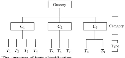
In this study, the class-based display policy is adopted. That is, items are allocated into shelf spaces based on their product category similarity first and then allocates items in the same product category into the shelf spaces based on their product type similarity. Let C = {C1, C2, …, CM} be the set of
product categories, where M is the total number of the product category and T = { T1, T2, …, TN} be the set of product types,
where N is the total number of product type. Fig. 1 shows an example of the hierarchal structure of item classification in this research. It is clear that C1= {T1, T2, T3, T4}, C2= {T5, T6,
T7}, and C3= {T8, T9
According to the above concept, the proposed shelf allocation framework is divided into two stages. The first
}.
Applying a Two-Stage Simulated Annealing
Algorithm for Shelf Space Allocation Problems
C1 C2 C3
T1 T5 T6
Category
Type
T2 T3 T4 T7 T8
Grocery
[image:2.595.306.541.48.221.2]T9
Fig. 1 The structure of item classification.
stage is to determine shelf space locations according to product category affinity information. In addition, the optimal shelf space location in product category level is resolved using the SA (Simulated Annealing) algorithm. After the shelf location in category level is determined, the second stage is to decide the shelf location in product type level in the same category. In this stage, product type association in the same category will be taken into consideration where the product type association can be derived according to retail’s trade database. Similar to the first stage, the SA algorithm is used to determine the shelf locations. The proposed research framework is summarized in Fig. 2. Due to paper length limitation, only stage one is introduced in the following sections.
B. The Formulation for the Shelf Allocation Problem
Let A=[ai,j] be the affinity matrix describing the affinity
relationship between categories where ai,j denotes the affinity
value between categories i and j. If affinity value between two categories is less than 0 and greater than -1, then the affinity between the two categories is adverse. If affinity value is 0 between two categories, then the affinity between the two categories is indifferent. As affinity value between two categories is less than 1 and greater than 0, then the affinity between two is affine. In addition, the distance between two product categories is evaluated by:
j i d D gh C h C g ij j i ≠ = ∈ ∈min, ,
(1)
where dgh
Locating product categories into shelves can be formulated as the objective function in (2) which is to maximize the sales profit and to maximize the affinity of every two product categories. (3) is the constraint that the total shelf spaces of category C
is the distance between the shelf space
g
andh.
i
i C
r
equals to . (4) is the constraint that each of shelf space only belongs to one category. (5) illustrates the constraint that shelf space numbers in the same category is uninterrupted and the cells are in number order.
h g j i D w PC b w PC b p P Max M j U k M i U g ij h j jh g i ig ij C ; , 1 1 1 1
≠ ≠ × × × × × × =
∑∑∑∑
= = = = (2) Subject to ; ..., , 2 , 1 , 1 M i r b U g Cig= i =
∑
= (3) ; ..., , 2 , 1 , 1 1 U g b M iig = =
∑
=(4)
To locate the shelf space of product
category To construct the
product category affinity matrix
To allocate the shelf space of product type To create association
clustering tree Retailer's
trade database
To develop the optimum of shelf allocation for retail
store
To adopt SA algorithm to solve location problem and
[image:2.595.65.265.50.143.2]allocation problem
Fig. 2 The overview of the proposed research framework.
; ..., , 2 , 1 , ..., , 2 , 1 ,
1 i M g U
b i i H L g
ig = = =
∏
=
(5)
where
M : the total number of the product category;
ig b : ; category product to belong not space shelf the , 1 ; category product to belong space shelf the , 0 i g i g jh b : ; category product to belong not space shelf the , 1 ; category product to belong space shelf the , 0 j h j h i
PC: the average profit per shelf space for the ith category;
j
PC : the average profit per shelf space for the jth
category;
g
w : the weight of shelf space g;
h
w : the weight of shelf space h;
,
, ,
if 0 , and the 4 -1 ,
= or 0 , and the 8
1 , otherwise
i j ij
i j i j ij
a D
p a D
< ≤
> >
{
| 1}
, 1 ,2 ,..., ;max g b i M
H ig
U g
i = ∈ = =
{
| 1}
, 1 ,2 ,..., .ming b i M
L ig
U g
i = ∈ = =
Note that
{
| 1}
i ig
g U
H max g b
∈
= = is the largest index number of
shelf space belongs to category Ci i
{
| ig 1}
g U
L min g b
∈
= =
, and
is the smallest index number of shelf space belongs to category Ci
C. Shelf Allocation using Simulated Annealing Algorithms
.
To solve the self space allocation problem in (2), this research uses SA algorithm with better initial salutation strategy, which is described as follows.
1) The coding scheme
1 2 3 4 5
6 7 8 9 10
Encode
[image:3.595.62.271.49.106.2]1 2 3 4 5 6 7 8 910
Fig. 3 The location numbers in a shelf encoded to the grid.
2) The initial parameters
The parameters used in SA algorithm are defined as follows:
T0 T
: initial temperature.
F: terminated temperature (T0 >TF and T0, TF T
≧0).
current
α: cooling rate.
: current temperature.
t: number of move.
tmax
The initial temperature is set according to the suggestion in which the initial temperature T
: maximum number of moves.
0 should yield an initial acceptance rate of at least 80% [12]. Therefore, the initial temperature is set to 100 in this research. The terminated temperature TF usually set as the value not less than zero
degrees. Kirkpatrick et al. [12] mentioned tmax is decided by
the number of decision variables multiplied by a constant factor where there are two decision variables big and bjh in this
case. The cooling rate α, which converts the temperature at each annealing temperature step, is set as a constant factor between 0.8 and 0.99 [12], [13]. After determining the above settings, current temperature Tcurrent is set as T0 and t as 1.
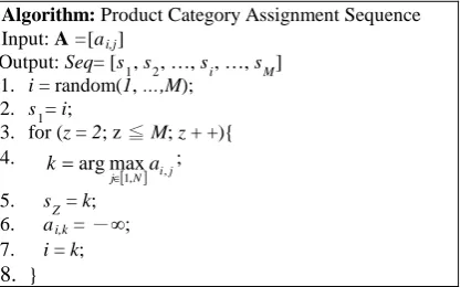
3) Initial solutions
In this research, an initial solution is derived based on consideration of affinity among product categories. Fig. 4 shows the pseudo-code of the proposed initial solution algorithm for product category. Let Seq = [s1, s2, …, si, …,
sM,] be product category assignment sequence where siis the product category number. As shown in lines 1 to 2, the algorithm first randomly selects one product category i and places at the first position of the sequence, s1
After executing this algorithm, an initial sequence for product category is obtained. Next, for each product category in Seq, we will obtain how many cell spaces in the product category and then add the desired of the product category into the grids. Finally, the initial solution PC will be obtained. In addition, the initial solution PC will be assigned as the current solution PC
. Then the product category having the largest affinity value with the product category i will be chosen as the second product category as shown in line 4 to 5. Furthermore, if the category j
is chosen as second category, affinity value between category
i and category j will become negative infinite. This assures that category j will not be chosen again. This process will be repeated until all product categories have been chosen as shown in line 4 to 8.
’ and the current best solution PC*.
4) Neighborhood solution search
This operator uses swapping strategy to produce a neighborhood solution PCt, which is close to current best solution PC*
Algorithm: Product Category Assignment Sequence
in search space. First, the operator randomly selects categories i and j in product category assignment sequence Seq to swap. Next, for each product category in Seq, we will obtain how many cell spaces in the product category and then add the desired of the product category into the grids.
Input: A =[ai,j
Output: Seq= [s
]
1, s2, …, si, …, sM
1. i = random(1, …,M);
]
2. s1
3. for (z = 2; z ≦ M; z + +){ = i;
4.
[ ] ij N
j a
k ,
, 1
max arg
∈
= ;
5. s
Z
6. a
= k;
i,k
7. i = k;
= -∞; 8. }
Fig. 4 The pseudo-code of the proposed Product Category Assignment Sequence (PCAS) Algorithm.
5) Acceptance probability
After deriving neighborhood solution PCt the algorithm needs to decide whether to accept this neighborhood solution or not. Let the change in the objective function value from PT*
to PCt, be defined as ΔEc = E(PC t
)-E(PC*) where E( ) denotes the objective function value of solution, refer to (3). If
ΔEc>0, the neighborhood solution PC t
is better than the current best solution PC*. Therefore, PC*= PCt . Oppositely, if ΔEc
≤
0, the algorithm will produce a random number Dranging from 0 to 1 and compare the random number D with a predefined acceptance probability PAC . The acceptance probability PAC is calculated as exp(-ΔEc/Tcurrent) where Tcurrent is the current temperature. If PAC > D, then this
neighborhood solution is kept and assigned as current solution PC’. That is, PC’= PCt. Otherwise, if PAC
≤
D the neighborhood solution PCt will not be accepted. If t does not reach the maximum number of moves tmax then the algorithmwill goes to back step 4 and generate another new neighborhood solution.
6) Cooling rate
The cooling rate α is the ratio of reduction from the former temperature to the new temperature. The new temperature will be calculated using the following equation:
current current
T
=
α
T
(6)7) Stopping criterion
If current temperature Tcurrent less than or equal to a
predetermined terminated temperature (TF), the SA algorithm
will stop; otherwise, goes back to step 4. After the stopping criterion is reached, the shelf space location for product category will be decoded.
III. EXPERIMENT RESULTS AND ANALYSIS
This section takes a simple case to demonstrate the feasible of the proposed shelf allocation method for a retail store. The retail store has a rectangular layout consisting of two aisles where width of every aisle is 2. There are totally 170 shelf spaces where width, length, and height of every shelf space are 1. Fig. 5 shows the retail store layout displayed in x and y
dimensions. Fig. 6 shows the 170 shelves displayed in x, y, and z dimensions and the weights for every cell. Note that length, width, and height of every shelf are 1, 1, and 5 respectively.
[image:3.595.307.516.50.180.2]12
ai sl e
2 ai
sl e
1 1 (1, 1)
(8, 7) 2
x y
(2, 12) (7, 12)
Area A Area B
Fig. 5 The retail store displayed in 2D.
0.4 0.6 0.4 0.2 0.1
0.4 0.6 0.4 0.2 0.1
0.4 0.6 0.4 0.2 0.1
0.4 0.6 0.4 0.2 0.1
0.4 0.6 0.4 0.2 0.1
0.4 0.6 0.4 0.2 0.1
1 2 1 0.8 0.6 0.7 0.9 0.7 0.5 0.3 0.6 0.8 0.6 0.4 0.2 0.5 0.7 0.5 0.3 0.1 0.6 0.8 0.6 0.4 0.2
ai
sl
e 1
0.7 0.9 0.7 0.5 0.3 1 2 1 0.8 0.6
1 2 1 0.8 0.6 0.7 0.9 0.7 0.5 0.3 0.6 0.8 0.6 0.4 0.2 0.5 0.7 0.5 0.3 0.1 0.6 0.8 0.6 0.4 0.2 1 0.7 0.6 0.5 0.6 0.7
1 2 1 0.8 0.6
0.7 0.9 0.7 0.5 0.3 1 2 1 0.8 0.6
aisle 2 1 2 1 0.8 0.6 0.7 0.9 0.7 0.5 0.3 0.6 0.8 0.6 0.4 0.2 0.5 0.7 0.5 0.3 0.1 0.6 0.8 0.6 0.4 0.2 0.7 0.9 0.7 0.5 0.3 1 2 1 0.8 0.6
X Y Z Upper layer
[image:4.595.56.552.33.586.2]Middle-upper layer Middle layer Middle-lower layer Lower layer
Fig. 6 The weight for every cell displayed in 3D.
munchies (C1)
drink (C2)
seasoning (C3)
booze (C4)
toy (C5)
housekeeping cleanser (C6)
facilities equipment (C7)
office stationery appliances (C8)
dried laver (T1)
candy (T2)
chocolate (T3)
cookies (T4)
salt (T6)
juice (T5)
wine (T7)
doll (T8)
robot (T9)
shampoo (T10)
soap (T11)
shredder (T12)
clip (T13)
desktop drawer (T14)
pen (T15)
[image:4.595.57.273.51.679.2]Grocery
Fig. 7 The item hierarchal structure.
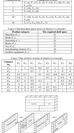
product categories and product types are shown in the parentheses. As shown in Table 1, there are thirty transaction records in this simple case. Note that the sales volume for every transaction product type is recorded in the parentheses. The required shelf space for each product category is obtained as shown in Table 2.
The relation between any two product categories is set up. Next, the affinity value of every two product categories will
TABLE 1THE TRANSACTION RECORDS OF THE TRANSACTION DATABASE.
Transaction ID Transaction records
1 T2 (4), T3 (17), T4 (9), T7 (14), T11 (20), T13 (9), T14
2
(20) T1 (18), T11 3
(5) T2 (14), T6 …
(16) …
29 T1 (18), T6 (2), T8 (1), T10 (12), T11 (4), T12 (6), T15
30
(5)
T1 (17), T10 (14), T11 (7)
TABLE 2THE REQUIRED SHELF SPACE OF PRODUCT CATEGORY.
Product category The required shelf space
Munchies (C1) 22
Drink (C2) 12
Seasoning (C3) 24
Booze (C4) 21
Toy (C5) 15
housekeeping cleanser (C6) 34
facilities equipment (C7) 27
TABLE 3THE AFFINITY MATRIX OF PRODUCT CATEGORY.
Category
No. C1 C2 C3 C4 C5 C6 C7 C
C
8 -
1 1 0.2 0.4 0.7 -1 0 0
C2 1 - 0.3 1 0 -1 0 0
C3 0.2 0.3 - 0.1 -0.5 -0.8 -0.5 -0.7
C4 0.4 1 0.1 - -0.1 -1 0.5 0
C5 0.7 0 -0.5 -0.1 - 0 0.5 -0.2
C6 -1 -1 -0.8 -1 0 - 0.2 0.5
C7 0 0 -0.5 0.5 0.5 0.2 - 1
C8 0 0 -0.7 0 -0.2 0.5 1 -
aisle 2 aisle 1
housekeeping cleanser
booze booze
office stationery
appliances facilities equipment toy
toy
munchies
seasoning seasoning drink
Fig. 8 The shelf location of the product category level.
be transformed into numerical, and these affinity values are created in affinity matrix as shown in Table 3. Note that the affinity value of every two product categories is established by managers.
[image:4.595.299.554.66.525.2] [image:4.595.59.276.407.677.2]TABLE 4THE RESULTS IN THE TWO SCENARIOS.
Adopting PCAS algorithm
Adopting Random method
1 17620.09 15384.09
2 17930.57 16091.10
3 16935.65 16168.91
4 17189.95 16665.32
5 17930.57 16665.32
6 16935.65 16935.65
7 16935.65 17189.95
8 17620.09 17519.77
9 16935.65 17519.769
10 17536.91 17930.567
Max 17930.567 17930.567
Min 16935.647 15384.092
Average 17357.076 16807.043
standard
deviation 417.2423 776.4711
Variance 174091.1 602907.3
After the shelf location in category level is determined, the second stage is to decide the shelf location in product type level in the same category. In this stage, product type association in the same category will be taken into consideration where the product type association can be derived according to retail’s trade database. Similar to the first stage, the SA algorithm is used to determine the shelf locations. After obtaining the maximum fitness, the assignment sequence of product type is decoded so that the allocation of these types into shelves is known. In this example, the maximum fitness is 40812.408 and its shelf allocation for each product type is shown in Fig. 9.
IV. CONCLUSIONS
In today’s highly competitive retail environment, retailers need to accurately and quickly respond the customers’ dynamic and ever-changing requirements. Shelf space arrangement is one of the most important issues in retailing. In retailing stores, different displaying strategies can directly influence customer’s purchasing decision and profit of retail stores. Effective product assignment and shelf space allocation can not only improve the profit of retail store but also attracted the customer’s attention and made good impression to the customers. This research proposes a two-stage shelf space allocation method that deals with product assignment and shelf space allocation problem simultaneously.
In this research, the shelf allocation problems using proposed a two-stage method can avoid the shortcomings of previous studies. The proposed two-stage shelf space allocation method takes many important points into consideration which are the customer buying behavior, the important weights of shelf spaces, the product category affinity, and purchasing association between product types. Besides, in the stage one, it is clear that the case of adopting PCAS algorithm has the better performance in fitness value and computation times when comparing to the case of adopting random method.
The proposed two-stage shelf allocation method can be improved further as following directions. First, the neighborhood solution search in the simulated annealing algorithm randomly selects two categories in product
aisle 2 aisle 1
wine wine
shredder doll
robot
salt
salt juice
shampoo soap
clip pen desktop
drawer
doll
robot
candy chocolate
[image:5.595.310.530.51.182.2]dried laver cookies
Fig. 9 The shelf allocation of the product type level.
category level to swap. In the future, different swap methods can be used in the operator strategy of neighborhood solution search. Second, how many items for specific product type each cell space stores can not be derived since the facing length, depth and height of the item and the cell space are not be considered. In the future, how to develop an appropriate stacking method to stack more items and the increase utilization of the shelf should be discussed further.
REFERENCES
[1] E.E. Anderson and H.N. Amato, “A mathematical model for simultaneously determining the optimal brand-collection and display-area allocation,” Operations Research, vol.22, 1974, pp. 13–21.
[2] N. Borin, P. W. Farris, and J. R. Freeland, “A model for determining retail product category assortment and shelf space allocation,” Decision Sciences, vol.25, 1994, pp. 359–384.
[3] M. Corstjens and P. Doyle, “A dynamic model for strategically allocating retail space,” Journal of the Operational Research Society, vol.34, 1983, pp. 943–951.
[4] T. L. Urban, “An inventory-theoretic approach to product assortment and shelf-space allocation,” Journal of Retailing, vol. 74, 1998, pp. 15–35.
[5] M. C. Chen and C.P. Lin, “A data mining approach to product assortment and shelf space allocation. Expert Systems with Applications, vol.32, 2007, pp. 976–986.
[6] C.Y. Tsai, M.J. Lin, and C.J. Chen, “An Efficient Assignment Sequence Algorithm for the Multi-Stage Shelf Allocation Problem,” Proceedings of the 8th APIEMS & 2007 CIIE Conference, Kaohsiung, Taiwan, 2007, December 9-13.
[7] X. Drèze, S.J. Hoch, M.E. Purk, “Shelf management and space elasticity,” Journal of Retailing, vol.70
[8] J. S. Larson, E. T. Bradlow, P. S. Fader, “An exploratory look at supermarket shopping paths,” International Journal of Research in Marketing, vol.22, 2005, 395–414.
, 1994, pp. 301–326.
[9] H. Hwang, B. Choi, M.J. Lee, “A model for shelf space allocation and inventory control considering location and inventory level effects on demand,” International Journal of Production Economics, vol.97, 2005, pp. 185–195.
[10] M.K. Maiti and M. Maiti, “Multi-item shelf-space allocation of breakable items via genetic algorithm,” Journal of Applied Mathematics and Computing, vol.20, 2006, pp. 327–343. [11] E. Van Nierop, D. Fok, and P.H. Franses. “Interaction between shelf
layout and marketing and its impact on optimizing shelf arrangements,” Marketing Science, vol.27, 2008, pp.1065–1082. [12] S. Kirkpatrick, C. D. Gelattt, and M. P. Vecchi, “Optimization by
Simulated Annealing,” Science, vol.220, 1983, pp. 671–680. [13] S. Kirkpatrick, “Optimization by simulated annealing: Quantitative
[image:5.595.45.268.53.241.2]