Co training and Self training for Word Sense Disambiguation

Co-training and Self-training for Word Sense Disambiguation

Rada Mihalcea

Department of Computer Science and Engineering

University of North Texas

[email protected]

Abstract

This paper investigates the application of co-training and self-co-training to word sense disam-biguation. Optimal and empirical parameter se-lection methods for co-training and self-training are investigated, with various degrees of error reduction. A new method that combines co-training with majority voting is introduced, with the effect of smoothing the bootstrapping learn-ing curves, and improvlearn-ing the average perfor-mance.

1

Introduction

The task of word sense disambiguation consists in assign-ing the most appropriate meanassign-ing to a polysemous word within a given context. Most of the efforts in solving this problem were concentrated so far towards supervised learning, where each sense tagged occurrence of a par-ticular word is transformed into a feature vector, which is then used in an automatic learning process. While these algorithms usually achieve the best performance, as compared to their unsupervised or knowledge-based al-ternatives, there is an important shortcoming associated with these methods: their applicability is limited only to those words for which sense tagged data is available, and their accuracy is strongly connected to the amount of la-beled data available at hand. In this paper, we investigate methods for building sense classifiers when only relatively few annotated examples are available. We explore boot-strapping methods using co-training and self-training, and evaluate their performance on the SENSEVAL-2 nouns. We show that classifiers built for different words have dif-ferent behavior during the bootstrapping process. If the right parameters for co-training and self-training can be identified (growth size, pool size, and number of itera-tions, as explained later in the paper), an average error reduction of 25.5% is achieved, with similar performance

observed for both co-training and self-training. However, with empirical settings, the error reduction is significantly smaller, with a 9.8% error rate reduction achieved for a new method that combines co-training with majority vot-ing.

We first overview the general approach of bootstrap-ping for natural language learning using co-training and self-training. We then introduce the problem of super-vised word sense disambiguation, and define several local and topical basic classifiers. We investigate the applica-bility of co-training and self-training to supervised word sense disambiguation, starting with these basic classifiers, and perform comparative evaluations of optimal and em-pirical bootstrapping parameter settings.

2

Co-training and Self-training for Natural

Language Learning

Co-training and self-training are bootstrapping methods that aim to improve the performance of a supervised learn-ing algorithm by incorporatlearn-ing large amounts of unlabeled data into the training data set.

2.1 Co-training

Starting with a set of labeled data, co-training algorithms (Blum and Mitchell, 1998) attempt to increase the amount of annotated data using some (large) amounts of unlabeled data. Shortly, co-training algorithms work by generating several classifiers trained on the input labeled data, which are then used to tag new unlabeled data. From this newly annotated data, the most confident predictions are sought, and subsequently added to the set of labeled data. The process may continue for several iterations.

One important aspect of co-training consists in the re-lation between the views used in learning. In the original definition of co-training, (Blum and Mitchell, 1998) state

conditional independence of the views as a required

cri-terion for co-training to work. In recent work, (Abney, 2002) shows that the independence assumption can be re-laxed, and co-training is still effective under a weaker in-dependence assumption. He is proposing a greedy algo-rithm to maximize agreement on unlabelled data, which produces good results in a co-training experiment for named entity classification. Moreover, (Clark et al., 2003) show that a naive co-training process that does not explic-itly seek to maximize agreement on unlabelled data can lead to similar performance, at a much lower computa-tional cost. In this work, we apply co-training by identify-ing two different feature sets based on a “local versus topi-cal” feature split, which represent potentially independent

views for word sense classification, as shown in Section 4.

2.2 Self-training

While there is a common agreement on the definition of co-training, the literature provides several sometimes conflicting definitions for self-training. (Ng and Cardie, 2003) define self-training as a “single-view weakly super-vised algorithm”, build by training a committee of clas-sifiers using bagging, combined with majority voting for final label selection. (Clark et al., 2003) provide a differ-ent definition: self-training is performed using “a tagger that is retrained on its own labeled cache on each round”. We adopt this second definition, which also agrees with the definition given in (Nigam and Ghani, 2000).

Self-training starts with a set of labeled data, and builds a classifier, which is then applied on the set of unlabeled data. Only those instances with a labeling confidence ex-ceeding a certain threshold are added to the labeled set. The classifier is then retrained on the new set of labeled examples, and the process continues for several iterations. Notice that only one classifier is required, with no split of features.

Figure 1 illustrates the general bootstrapping process. Starting with a set of labeled and unlabeled data, the boot-strapping algorithm aims to improve the classification performance, by integrating examples from the unlabeled data into the labeled data set. At each iteration, the class distribution in the labeled data is maintained, by keeping a constant ratio across classes between already labeled examples and newly added examples; the role of this step is to avoid introducing imbalance in the training data set. For co-training, the algorithm requires two different views (two different classifiers

and

) that interact in the bootstrapping process. By limiting the number of views to one (one general classifier

), co-training is transformed into a self-training process, where one single classifier learns from its own output.

0. Given:

- A set L of labeled training examples - A set U of unlabeled examples - Classifiers

1. Create a pool U’ of examples by choosing P random ex-amples from U

2. Loop for I iterations:

2.1 Use L to individually train the classifiers

, and

la-bel the examples in U’

2.2 For each classifier select G most confidently

ex-amples and add them to L, while maintaining the class distribution in L

2.3 Refill U’ with examples from U, to keep U’ at a con-stant size of P examples

Figure 1: General bootstrapping process using labeled and unlabeled data

Co-training and self-training parameters

Three different parameters can be set in the bootstrapping process, and usually the performance achieved through bootstrapping depends on the value chosen for these pa-rameters.

Iterations (I) Number of iterations.

Pool size (P) Number of examples selected from the

unlabeled set U for annotation at each iteration.

Growth size (G) Number of most confidently labeled

examples that are added at each iteration to the set of labeled data L.

As previously noticed (Ng and Cardie, 2003), there is no principled method for selecting optimal values for these parameters, which is an important disadvantage of these algorithms. In the following, we show that there is a big gap between the performance achieved for some op-timal parameter settings, selected through measurements performed on the test data, and the performance level when these parameters are set empirically, suggesting that more research is required to narrow this gap, and make these bootstrapping algorithms useful for practical appli-cations.

First, we describe the general framework of supervised word sense disambiguation, and introduce several basic sense classifiers that are used in co-training and self-training experiments. Next, through several experiments, (1) we determine the optimal parameter settings for co-training and self-co-training, and (2) explore various algo-rithms for empirical selection of these three parameters for best performance.

3

Supervised Word Sense Disambiguation

available for a target ambiguous word. These examples are used to build a classifier that automatically learns clues useful for the disambiguation of the given polysemous word, and then applies these clues to the classification of new unlabeled instances.

First, the examples are pre-processed and annotated with morphological or syntactic tags. Next, each sense-tagged example is transformed into a feature vector, suit-able for an automatic learning process. There are two main decisions that one takes in the construction of such a classifier: (1) What features to extract from the exples provided, to best model the behavior of the given am-biguous word; (2) What learning algorithm to use for best performance.

3.1 Preprocessing

During preprocessing, SGML tags are eliminated, the text is tokenized and annotated with parts of speech. Collo-cations are identified using a sliding window approach, where a collocation is considered to be a sequence of words that forms a compound concept defined in Word-Net. During this process, all collocations that include the target word are identified, and the examples that use a collocation are removed from the training/test data. For instance, examples referring to short circuit are removed from the data set for circuit, so that a separate learning process is performed for each lexical unit.

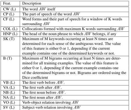
Feat. Description CW (L) The word itself

CP (L) The part of speech of the word

CF (L) Word forms and their part of speech for a window of K words surrounding

COL (L) Collocations formed with maximum K words surrounding

HNP (L) The head of the noun phrase to which belongs, if any

SK (T) Maximum of M keywords occurring at least N times are determined for each sense of the ambiguous word. The value of this feature is either 0 or 1, depending if the current example contains one of the determined keywords or not. B (T) Maximum of M bigrams occurring at least N times are

deter-mined for all training examples. The value of this feature is either 0 or 1, depending if the current example contains one of the determined bigrams or not. Bigrams are ordered using the Dice coefficient

VB (L) The first verb before .

VA (L) The first verb after .

NB (L) The first noun before .

NA (L) The first noun after .

VO (L) Verb-object relation involving

SV (L) Subject-verb relation involving

Table 1: Commonly used features for word sense disam-biguation.

denotes the current (ambiguous) word. Feature type is indicated as local (L) or topical (T).

3.2 Features that are good indicators of word sense

Previous work on word sense disambiguation has ac-knowledged several local and topical features as good in-dicators of word sense. These include surrounding words and their part of speech tags, collocations, keywords in

contexts. More recently, other possible features have been investigated: bigrams, named entities, syntactic features, semantic relations with other words in context. Table 1 lists commonly used features in word sense disambigua-tion (list drawn from a larger set of features compiled by (Mihalcea, 2002)).

3.3 Supervised learning for word sense disambiguation

Related work in supervised word sense disambigua-tions includes experiments with a variety of learning algorithms, with varying degrees of success, including Bayesian learning, decision trees, decision lists, memory based learning, and others. (Yarowsky and Florian, 2002) give a comprehensive examination of learning methods and their combination.

3.4 Basic Classifiers for Word Sense Disambiguation

Several basic word sense disambiguation classifiers can be implemented using feature combinations from Table 1, and feature vectors can be plugged into any learning algo-rithm. We use Naive Bayes, since it was previously shown that in combination with the features we consider, can lead to a state-of-the-art disambiguation system (Lee and Ng, 2002). Moreover, Naive Bayes is particularly suitable for co-training and self-training, since it provides confidence scores and is efficient in terms of training and testing time. The two separate views required for co-training are de-fined using a local versus topical feature split. For self-training, a global classifier with no feature split is defined. A local classifier

A local classifier was implemented using all local features listed in Table 1.

A topical classifier

The topical classifier relies on features extracted from a large context, in particular keywords specific to each indi-vidual sense. We use the SK feature, and extract at most ten keywords for each word sense, each occurring for at least three times in the annotated corpus.

A global classifier

Finally, the global classifier integrates all local and topical features, also in a Naive Bayes classifier. This classifier is basically a combination of the previous two local and topical classifiers.

4

Co-training and Self-training for Word

Sense Disambiguation

We investigate the application of co-training and self-training to the problem of supervised word sense disam-biguation, and explore methods for selecting values for the bootstrapping parameters.

to these data sets, a large raw corpus of unlabeled exam-ples is constructed for each word, with text snippets con-sisting of three consecutive sentences extracted from the British National Corpus. Given the large number of runs performed for each word, the experiments focus on nouns only. Similar observations are however expected to hold for other parts of speech.

For co-training, we use the local and topical classifiers described in Section 3.4, which represent two different views for this problem, generated by a “local versus top-ical” feature split. Self-training requires only one basic classifier, and we use a global classifier, which combines the features from both local and topical views for a com-plete global “view”.

Unlike previous applications of co-training and self-training to natural language learning, where one general classifier is build to cover the entire problem space, su-pervised word sense disambiguation implies a different classifier for each individual word, resulting eventually in thousands of different classifiers, each with its own characteristics (learning rate, sensitivity to new examples, etc.). Given this heterogeneous space of classifiers, our hypothesis is that co-training and self-training will them-selves have a heterogeneous behavior, and therefore best co-training and self-training parameters are different for each classifier.

To explore this hypothesis, a range of experiments is performed. First, for all the words in the experimental data set, an optimal parameter setting is determined. This can be considered as an upper bound for improvements achieved with co-training and self-training, since the se-lection of parameters is performed through measurements that are collected directly on test data. Second, we explore several algorithms to select the bootstrapping parameters, independent of the test set: (1) Best overall parameter set-ting; (2) Best individual parameter settings; (3) Best per-word parameter selection; (4) A new method consisting in an improved bootstrapping scheme using majority voting across several bootstrapping iterations.

4.1 Optimal settings

Optimal parameter settings are determined through mea-surements performed directly on the test set. For the growth size G, a value is chosen from the set: 1, 10, 20, 30, 40, 50, 100, 150, 200 . The pool size P takes one of these values: 1, 100, 500, 1000, 1500, 2000, 5000 . For each setting, 40 iterations are performed. This results in an average of 2,120 classification runs per word. At each run, a pool of P raw examples is annotated, and G most confidently labeled examples are added to the training set from the previous iteration. The performance of the clas-sifier using the augmented training set is evaluated on the test data, and the precision is recorded.

Separate experiments are performed for both

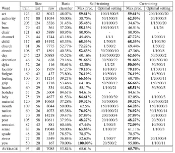
co-training and self-co-training, for all the nouns in the SENSEVAL-2 data set (for a total of about 120,000 runs). For each word, the parameter setting (growth size G / pool size P / iterations I) leading to the highest improvement is determined. Table 21 lists, for each word: size of train-ing, test, raw data2; precision of the basic classifier (the global classifier is used as a baseline); maximum preci-sion obtained with co-training and self-training, and the parameters for which this maximum is achieved. When several parameter settings lead to the same performance, the first setting is recorded.

Discussion

Surprisingly, under optimal settings, both co-training and self-training perform about the same, leading to an aver-age error reduction of 25.5%. Self-training leads to the highest precision for nine words, while co-training is win-ning for eight words; there is a tie with equal performance for both co-training and self-training for the remaining twelve words.

There are three words (chair, holiday, spade) for which no improvement could be obtained with either co-training or self-training, and therefore no optimal setting is indi-cated. These are among the four words with the best per-forming basic classifier (baseline higher than 75%). The fact that no improvement was obtained agrees with previ-ous observations that classifiers that are too accurate can-not be improved with bootstrapping (Pierce and Cardie, 2001). Note that even very weak classifiers, with preci-sions below 40%, can still be improved, sometimes with as much as 45% error reduction (e.g. the classifier for

feeling).

There are no clear commonalities between the param-eters leading to maximum precision for different classi-fiers. Some classifiers benefit more from an “aggressive” augmentation of the training data with new examples – for instance the self-trained classifier for nature achieves its highest peak for a growth size of 200 from a pool of 500 examples. Others instead work better by taking “short steps” – for instance self-training for the word dyke works better for a growth size of 1 from a pool of 1.

1

The numbers listed in Table 2 for training/test data size and basic classifier precision refer to data sets obtained after remov-ing examples with collocations that include the target word. This explains why the numbers do not always match figures previ-ously reported in SENSEVAL-2 literature. If collocations are added back to the data sets, the precision of the basic classifier is measured at 60.2% – comparable to figures obtained by other systems participating in SENSEVAL-2

2

Size Basic Self-training Co-training Word train test raw classifier Max.prec. Optimal setting Max.prec. Optimal setting

art 123 52 8012 48.07% 59.61% 100/1500/5 59.61% 200/1000/20 authority 157 80 11034 50.00% 58.75% 50/1500/3 62.50% 20/1000/3 bar 205 124 5526 31.45% 35.48% 10/1000/3 34.67% 1/1500/20 bum 79 43 361 37.20% 58.13% 100/100/13 46.51% 1/1/26

chair 121 63 5889 80.95% 80.95% - 80.95%

-channel 78 44 1744 43.18% 45.45% 1/1/1 47.72% 1/2000/1 child 117 60 14192 63.33% 68.33% 1/500/3 68.33% 1/100/30 church 81 36 7775 52.77% 72.22% 1/500/2 69.44% 1/500/2 circuit 108 57 1891 40.35% 52.63% 30/2000/10 47.36% 1/100/8 day 245 123 50883 45.52% 60.16% 100/5000/20 62.60% 50/5000/2 detention 46 24 638 79.16% 91.66% 30/500/22 91.66% 100/500/10 dyke 52 26 116 38.61% 42.30% 1/1/23 50.00% 50/500/1 facility 110 55 1959 67.27% 78.18% 10/100/3 78.18% 1/1500/11 fatigue 69 42 437 73.80% 76.19% 10/500/1 76.19% 10/500/1 feeling 100 51 11214 39.21% 66.66% 1/2000/6 60.78% 1/2000/11 grip 72 39 1718 53.46% 64.10% 50/500/12 66.66% 150/500/1 hearth 60 29 334 44.82% 55.17% 1/100/21 65.51% 50/500/3

holiday 55 26 5604 84.61% 84.61% - 84.61%

-lady 75 39 4677 61.53% 84.61% 20/100/39 82.05% 1/1000/3 material 120 59 10663 37.28% 59.32% 50/5000/6 59.32% 100/5000/24 mouth 109 56 8044 50.00% 62.5% 150/1000/3 64.28% 150/1000/3 nation 60 26 4073 65.38% 76.92% 40/1000/21 76.92% 30/1500/14 nature 70 38 14218 39.47% 57.89% 200/500/4 57.89% 30/1000/3 post 105 58 10611 37.93% 48.27% 20/1000/3 48.27% 20/500/1 restraint 87 43 881 60.46% 67.44% 1/500/5 72.09% 10/500/1 sense 83 36 19048 50.00% 63.88% 1/100/37 61.11% 1/100/3

spade 48 28 235 78.57% 78.57% - 78.57%

-stress 77 38 3549 36.84% 52.63% 1/500/7 57.89% 20/1500/4 yew 50 20 167 70.00% 100.00% 20/500/2 95.00% 1/100/11 AVERAGE 95 48 7085 53.84% 65.61% - 65.75%

-Table 2: Size of training, test, and raw data, precision of basic classifiers, and maximum precision obtained for optimal parameter settings for self-training and co-training. The optimal settings column lists the values for the three parameters (growth size G / pool size P / iteration I) for which the maximum precision was observed.

The improvements obtained under these optimal set-tings can be considered as an upper bound for self-training and co-training. Under some ideal conditions, where the optimal parameters can be identified, this is the highest improvement that can be achieved for the given labeled set. However, most of the times, it may not be possible to find these optimal parameter values. In the following, we explore empirical solutions for finding values for these parameters, independent of the test data.

4.2 Empirical Settings

The methods described in this section make use of the data collected during self-training and co-training runs, for dif-ferent parameter settings. Evaluations are performed on a validation set consisting of about 20% of the training data – which was set apart for this purpose. For each run, infor-mation is collected about: initial size of labeled data set, growth size, pool size, iteration number, precision of basic classifier, precision of boosted classifier. With the range of values for growth size, pool size, and number of itera-tions specified in Section 4.1, about 60,000 such records are collected for both co-training and self-training.

4.2.1 Best overall parameter setting

One simple method to select a parameter setting is to determine a global setting that leads to the highest overall boost in precision. Starting with the information collected for the 60,000 runs, for each possible parameter setting, the total relative growth in performance is determined, by adding up the relative improvements for all the runs for that particular setting. For co-training, the best global set-ting identified in this way is growth size of 50, pool size of 5000, iteration 2. For self-training, the best setting is growth size of 1, pool size of 1500, iteration 2. The pre-cision obtained for these settings is listed in Table 3 un-der the global settings column. On average, using this scheme for parameter selection, co-training brings 4% er-ror reduction, while self-training has only a small erer-ror reduction of 1%.

Basic Global setting Per-word setting

Word classifier co-train self-train co-train setting self-train setting

art 48.07% 53.85% 50.00% 44.23% 50/1500/32 34.67% 10/100/1 authority 50.00% 51.25% 50.00% 57.50% 150/2000/2 37.50% 30/2000/3 bar 31.45% 31.45% 31.45% 29.83% 10/1000/5 24.19% 150/1000/17 bum 37.20% 39.53% 41.86% 46.51% 1/1/40 46.51% 1/1/34 chair 80.95% 77.78% 77.78% 77.77% 1/1500/16 76.19% 30/100/1 channel 43.18% 34.09% 43.18% 43.18% 1/2000/2 43.18% 1/2000/3 child 63.33% 50.00% 60.00% 55.00% 10/1500/1 53.33% 50/1500/17 church 52.77% 55.56% 58.33% 47.22% 1/100/23 55.55% 1/100/10 circuit 40.35% 45.61% 40.35% 31.57% 100/100/3 42.10% 1/1000/18 day 45.52% 52.03% 39.84% 50.43% 150/1500/3 49.59% 10/200/40 detention 79.16% 83.33% 79.17% 79.16% - 79.16% -dyke 38.61% 50.00% 38.46% 34.61% 1/2000/19 34.61% 1/2000/11 facility 67.27% 69.09% 72.73% 58.18% 150/1500/13 70.9% 100/100/7 fatigue 73.80% 71.43% 71.43% 71.43% 1/1000/1 71.43% 1/500/9 feeling 39.21% 39.21% 37.25% 50.98% 10/500/5 33.33% 1/500/25 grip 53.46% 43.59% 51.28% 41.02% 20/100/20 58.97% 40/100/40 hearth 44.82% 48.28% 44.82% 41.37% 1/1000/2 44.82% 1/2000/1 holiday 84.61% 84.61% 84.61% 84.61% - 84.61% -lady 61.53% 74.36% 58.97% 33.07% 150/2000/10 69.23% 100/500/40 material 37.28% 45.76% 40.68% 45.76% 100/2000/6 30.50% 10/2000/9 mouth 50.00% 51.79% 50.00% 53.57% 1/1/40 50.00% 20/2000/17 nation 65.38% 69.23% 57.69% 69.23% 100/2000/23 61.53% 150/2000/16 nature 39.47% 50.00% 42.11% 44.73% 10/100/3 50.00% 200/2000/34 post 37.93% 44.82% 39.66% 44.82% 1/500/28 36.20% 10/100/2 restraint 60.46% 58.14% 58.14% 53.48% 1/1000/2 62.79% 1/1000/15 sense 50.00% 47.22% 50.00% 25.00% 150/500/40 47.22% 1/2000/12

spade 78.57% 75.00% 78.57% 78.57% - 78.57%

-stress 36.84% 52.63% 47.37% 47.36% 1/1500/7 36.84% 10/1000/1

yew 70.00% 65.00% 75.00% 70.00% - 70.00%

-AVERAGE 53.84% 55.67% 54.16% 51.73% - 52.88%

-Table 3: Precision obtained with co-training and self-training, for global and per-word parameter selection.

parameters are growth size of 1, pool size of 1, iteration 1 (i.e. the best classifier is the one “closest” to the basic classifier). The average results are however worse than the baseline – only 53.49% for co-training, and 53.67% for self-training.

4.2.2 Best per-word parameter setting

In a second experiment, best parameter settings are identified separately for each word. The setting yielding to maximum precision on the validation set is selected as the best setting for a given word, and evaluated on the test data. If multiple settings are identified as leading to max-imum precision, settings are prioritized based on (in this order): smallest growth size; largest pool size; number of iterations. Results for both co-training and self-training are listed in Table 3 under the per-word settings column, together with the setting identified as optimal on the val-idation set. There are several words for which significant improvement is observed over the baseline. However, on the average, the performance of the boosted classifiers is worse than the baseline.

4.2.3 Smoothed co-training and self-training with majority voting

There is a common trend observed for learning curves for co-training or self-training, consisting in an increase

in performance followed by a decline. Different classi-fiers exhibit however a different point of raise or decline in precision, depending on the number of iterations. For instance, the classifier for circuit achieves its highest peak at iteration 10 (see Table 2), while the classifier for nation has the highest boost at iteration 21 – where the perfor-mance for circuit is already below the baseline. Given this heterogeneous behavior, it is difficult to identify a point of maximum for each classifier, or at least a point where the performance is not below the baseline. Ideally, we would like the learning curves to have a more stable behavior – without sharp raises or drops in precision, and with larger intervals with constant performance, so that the chance of selecting a good number of iterations for each classifier is increased.

We introduce a new bootstrapping scheme that com-bines co-training or self-training with majority voting. During the bootstrapping process, the classifier at each it-eration is replaced with a majority voting scheme applied to all classifiers constructed at previous iterations. This change has the effect of “smoothing” the learning curves: it slows down the learning rate, but also yields a larger interval with constant high performance3_.

3

35 40 45 50 55 60 65

0 5 10 15 20 25 30 35 40

Precision (%)

Number of iterations

Learning curves for simple and smoothed co-training

simple co-training smoothed co-training baseline

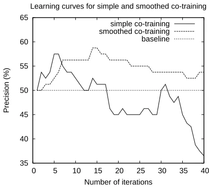
Figure 2: Learning curves for the classifier for the noun

authority: baseline, simple co-training, and co-training

smoothed with majority voting.

To some extent, smoothed co-training is related to boosting, since both algorithms rely on a growing ensem-ble of classifiers trained on resamples of the data. How-ever, boosting assumes labeled data and is error-driven, whereas smoothed co-training combines both labeled and unlabeled data and is confidence-driven4_.

Figure 2 shows the learning curves for simple co-training, and co-training “smoothed” with majority vot-ing, for the word authority (for a growth size of 1 and pool size of 1). Notice that the trend for the smoothed curve is still the same – a raise, followed by a decline – but at a significantly lower pace. With smoothed co-training, any number of iterations selected in the interval 5-40 still leads to significant improvement over the baseline, unlike the simple unsmoothed curve, where only iterations in the range 3-10 bring improvement over the baseline (followed by two other iterations at random intervals).

The methods for global parameter settings and per-word parameter settings are evaluated again, this time us-ing smoothed co-trainus-ing or self-trainus-ing. Table 4 lists the results obtained with basic and smoothed co-training for the same global/per-word setting. Since the major-ity voting scheme requires an odd number of classifiers,

sifiers across co-training iterations, with the effect of

improv-ing the performance of basic co-trainimprov-ing. This is

fundamen-tally different from the approach proposed in (Ng and Cardie, 2003), where they also apply majority voting in a bootstrapping framework, but in a different setting. They use a majority voting scheme applied to classifiers build on subsets of the labeled data (bagging) to induce several views for the co-training process. In their approach, majority voting is used at each co-training itera-tion to enable co-training by predicting labels on unlabeled data.

4

Thanks to one of the anonymous reviewers for suggesting this analogy.

Global setting Per-word setting Basic Co-training Co-training Word classifier basic smoothed basic smoothed

art 48.07% 53.85% 53.85% 44.23% 53.85% authority 50.00% 51.25% 57.50% 57.50% 58.75% bar 31.45% 31.45% 31.45% 29.83% 35.48% bum 37.20% 39.53% 44.18% 46.51% 44.18% chair 80.95% 77.78% 79.36% 77.78% 80.95% channel 43.18% 34.09% 43.18% 43.18% 45.45% child 63.33% 50.00% 51.66% 55.00% 65.00% church 52.77% 55.56% 58.33% 47.22% 58.33% circuit 40.35% 45.61% 49.12% 31.57% 42.10% day 45.52% 52.03% 53.65% 50.43% 55.28% detention 79.16% 83.33% 83.33% 79.16% 79.16% dyke 38.61% 50.00% 46.15% 34.61% 38.46% facility 67.27% 69.09% 69.09% 58.18% 58.18% fatigue 73.80% 71.43% 71.43% 71.43% 71.43% feeling 39.21% 39.22% 50.98% 50.98% 35.29% grip 53.46% 43.59% 48.71% 41.02% 60.00% hearth 44.82% 48.28% 44.82% 41.37% 44.82% holiday 84.61% 84.61% 84.61% 84.61% 84.61% lady 61.53% 74.36% 76.92% 33.07% 66.66% material 37.28% 45.76% 42.37% 45.76% 49.15% mouth 50.00% 51.79% 57.14% 53.57% 50.00% nation 65.38% 69.23% 69.23% 69.23% 73.07% nature 39.47% 50.00% 47.36% 44.73% 47.36% post 37.93% 44.83% 48.27% 44.82% 41.37% restraint 60.46% 58.14% 60.46% 53.48% 60.46% sense 50.00% 47.22% 58.34% 25.00% 33.33% spade 78.57% 75.00% 78.57% 78.57% 78.57% stress 36.84% 52.63% 55.26% 47.36% 52.63% yew 70.00% 65.00% 75.00% 70.00% 70.00%

AVERAGE 53.84% 55.67% 58.35% 51.73% 56.68%

Table 4: Basic and smoothed co-training, with global and per-word parameter settings (same settings as listed in Ta-ble 3)

the number of iterations is rounded up to the next even number (the first iteration is iteration 0, representing the basic classifier, which is also considered during voting). The same type of experiments were also performed for self-training, but the majority voting scheme did not bring any significant improvements. We believe that the learn-ing curves for self-trainlearn-ing are less steep, and therefore majority voting applied to classifiers across various itera-tions does not have the same strong smoothing effect as with co-training.

Discussion

in (Abney, 2002), and then empirically in (Clark et al., 2003), co-training still works under a weaker indepen-dence assumption, and the results we obtain concur with these previous observations.

Despite the fact that parameters observed for optimal settings (Table 2) are different for each classifier, in em-pirical settings, one unique set of parameters for all clas-sifiers seems to perform better than an individual set of parameters customized to each word. The bootstrapping scheme is improved even more when coupled with ma-jority voting across various iterations. Overall, the high-est error reduction is achieved with smoothed co-training using global parameter settings, where an average error reduction of 9.8% is observed with respect to the basic classifier.

A comparative analysis of words that benefit from ba-sic/smoothed co-training with global parameter settings, versus words with little or no improvement obtained through bootstrapping reveals several observations: (1) Words with accurate basic classifiers cannot be im-proved through co-training, which agrees with previous observations (Pierce and Cardie, 2001). For instance, no improvement was obtained for chair, holiday, or spade, which have the basic classifier performing above 75%. (2) Words with high number of senses (e.g. bar – 10 senses, channel – 7 senses, grip – 11 senses) achieve min-imal improvements through co-training. This is probably explained by the fact that the classifiers are misled by the large number of classes (senses), and a large number of errors is introduced since the early stages of co-training. (3) Words that have a large number of senses not belong-ing to well-defined topical domains show little or no ben-efit from a bootstrapping procedure. Using the domains attached to word senses, as introduced in (Magnini et al., 2002), we observed that words that have a large subset of their senses not belonging to a specific domain (e.g.

re-straint, facility) achieve little or no improvement through

co-training, which is perhaps explained again by the noisy automatic annotation that introduces errors since the early iterations of co-training.

Even though not all words show benefit from co-training, smoothed co-training with global parameter set-tings does bring an overall error reduction of 9.8% with respect to the basic classifier, which proves that bootstrap-ping through co-training is a potentially useful technique for word sense disambiguation.

5

Conclusion

This paper investigated the application of co-training and self-training to supervised word sense disambiguation. If the right parameters for co-training and self-training can be identified for each individual classifier, an average error reduction of 25.5% is achieved, with similar performance observed for both co-training and self-training. Given

that these optimal settings cannot always be identified in practical applications, several algorithms for empirical pa-rameter selection were investigated: global settings de-termined as the best set of parameters across all classi-fiers, and per-word settings, identified separately for each classifier, both using a validation set. An improved training method was also introduced, that combines co-training with majority voting, with the effect of smooth-ing the learnsmooth-ing curves, and improvsmooth-ing the average perfor-mance. This improved co-training algorithm, applied with a global parameter selection scheme, brought a significant error reduction of 9.8% with respect to the basic classi-fier, which shows that co-training can be successfully em-ployed in practice for bootstrapping sense classifiers.

Acknowledgments

Many thanks to Carlo Strapparava and the three anony-mous reviewers for useful comments and suggestions. This work was partially supported by a National Science Foundation grant IIS-0336793.

References

S. Abney. 2002. Bootstrapping. In Proceedings of the 40st Annual Meeting

of the Association for Computational Linguistics ACL 2002, pages 360–367,

Philadelphia, PA, July.

A. Blum and T. Mitchell. 1998. Combining labeled and unlabeled data with co-training. In COLT: Proceedings of the Workshop on Computational Learning

Theory, Morgan Kaufmann Publishers.

S. Clark, J. R. Curran, and M. Osborne. 2003. Bootstrapping POS taggers using unlabelled data. In Walter Daelemans and Miles Osborne, editors, Proceedings

of CoNLL-2003, pages 49–55. Edmonton, Canada.

Y.K. Lee and H.T. Ng. 2002. An empirical evaluation of knowledge sources and learning algorithms for word sense disambiguation. In Proceedings of the 2002

Conference on Empirical Methods in Natural Language Processing (EMNLP 2002), pages 41–48, Philadelphia, June.

B. Magnini, C. Strapparava, G. Pezzulo, and A. Gliozzo. 2002. Using domain in-formation for word sense disambiguation. In Proceedings of Senseval-2

Work-shop, Association of Computational Linguistics, pages 111–115, Toulouse,

France.

R. Mihalcea. 2002. Instance based learning with automatic feature selection ap-plied to Word Sense Disambiguation. In Proceedings of the 19th International

Conference on Computational Linguistics (COLING-ACL 2002), Taipei,

Tai-wan, August.

V. Ng and C. Cardie. 2003. Weakly supervised natural language learning without redundant views. In Human Language Technology/Conference of the North

American Chapter of the Association for Computational Linguistics (HLT-NAACL), Edmonton, Canada, May.

K. Nigam and R. Ghani. 2000. Analyzing the effectiveness and applicability of co-training. In Proceedings of the Conference on Information and Knowledge

Management CIKM-2000, pages 86–93, McLean, Virginia.

D. Pierce and C. Cardie. 2001. Limitations of co-training for natural language learning from large datasets. In Proceedings of the 2001 Conference on

Em-pirical Methods in Natural Language Processing (EMNLP-2001), Pittsburgh,

PA.

A. Sarkar. 2001. Applying cotraining methods to statistical parsing. In

Proceed-ings of the North American Chapter of the Association for Compuatational Linguistics, NAACL 2001, Pittsburg, June.

D. Yarowsky and R. Florian. 2002. Evaluating sense disambiguation across di-verse parameter spaces. JNLE Special Issue on Evaluating Word Sense