Scalable Term Selection for Text Categorization
Jingyang Li
National Lab of Intelligent Tech. & Sys. Department of Computer Sci. & Tech.
Tsinghua University, Beijing, China
Maosong Sun
National Lab of Intelligent Tech. & Sys. Department of Computer Sci. & Tech.
Tsinghua University, Beijing, China
Abstract
In text categorization, term selection is an important step for the sake of both cate-gorization accuracy and computational ef-ficiency. Different dimensionalities are ex-pected under different practical resource re-strictions of time or space. Traditionally in text categorization, the same scoring or ranking criterion is adopted for all target dimensionalities, which considers both the discriminability and the coverage of a term, such asχ2or IG. In this paper, the poor ac-curacy at a low dimensionality is imputed to the small average vector length of the docu-ments. Scalable term selection is proposed to optimize the term set at a given dimen-sionality according to an expected average vector length. Discriminability and cover-age are separately measured; by adjusting the ratio of their weights in a combined cri-terion, the expected average vector length can be reached, which means a good com-promise between the specificity and the ex-haustivity of the term subset. Experiments show that the accuracy is considerably im-proved at lower dimensionalities, and larger term subsets have the possibility to lower the average vector length for a lower com-putational cost. The interesting observations might inspire further investigations.
1 Introduction
Text categorization is a classical text information processing task which has been studied adequately
(Sebastiani, 2002). A typical text categorization pro-cess usually involves these phases: document in-dexing, dimensionality reduction, classifier learn-ing, classification and evaluation. The vector space model is frequently used for text representation (document indexing); dimensions of the learning space are calledterms, orfeaturesin a general ma-chine learning context. Term selection is often nec-essary because:
• Manyirrelevantterms have detrimental effect on categorization accuracy due to overfitting (Sebastiani, 2002).
• Some text categorization tasks have many rel-evant but redundant features, which also hurt the categorization accuracy (Gabrilovich and Markovitch, 2004).
• Considerations on computational cost:
(i) Many sophisticated learning machines are very slow at high dimensionalities, such as LLSF (Yang and Chute, 1994) and SVMs. (ii) In Asian languages, the term set is often very large and redundant, which causes the learning and the predicting to be really slow. (iii) In some practical cases the computational resources (time or space) are restricted, such as hand-held devices, real-time applications and frequently retrained systems. (iv) Some deeper analysis or feature reconstruction techniques rely on matrix factorization (e.g. LSA based on SVD), which might be computationally in-tractable while the dimensionality is large. Sometimes an aggressive term selection might be needed particularly for (iii) and (iv). But it is no-table that the dimensionality is not always directly
connected to the computational cost; this issue will be touched on in Section 6. Although we have many general feature selection techniques, the do-main specified ones are preferred (Guyon and Elis-seeff, 2003). Another reason for ad hoc term se-lection techniques is that many other pattern clas-sification tasks has no sparseness problem (in this study the sparseness means a sample vector has few nonzero elements, but not the high-dimensional learning space has few training samples). As a ba-sic motivation of this study, we hypothesize that the low accuracy at low dimensionalities is mainly due to the sparseness problem.
Many term selection techniques were presented and some of them have been experimentally tested to be high-performing, such as Information Gain,χ2 (Yang and Pedersen, 1997; Rogati and Yang, 2002) and Bi-Normal Separation (Forman, 2003). Every-one of them adopt a criterion scoring and ranking the terms; for a target dimensionalityd, the term se-lection is simply done by picking out the top-dterms from the ranked term set. These high performing cri-teria have a common characteristic — both discrim-inability and coverage are implicitly considered.
• discriminability: how unbalanced is the distri-bution of the term among the categories.
• coverage: how many documents does the term occur in.
(Borrowing the terminologies from document index-ing, we can say the specificity of a term set corre-sponds to the discriminability of each term, and the exhaustivity of a term set corresponds to the cov-erage of each term.) The main difference among these criteria is to what extent the discriminability is emphasized or the coverage is emphasized. For in-stance, empiricallyIGprefers high frequency terms more thanχ2does, which meansIGemphasizes the coverage more thanχ2does.
The problem is, these criteria are nonparametric and do the same ranking for any target dimensional-ity. Small term sets meet the specificity–exhaustivity dilemma. If really the sparseness is the main rea-son of the low performance of a small term set, the specificity should be moderately sacrificed to im-prove the exhaustivity for a small term set; that is to say, the term selection criterion should consider coverage more than discriminability. Contrariwise, coverage could be less considered for a large term
set, because we need worry little about the sparse-ness problem and the computational cost might de-crease.
The remainder of this paper is organized as fol-lows: Section 2 describes the document collections used in this study, as well as other experiment set-tings; Section 3 investigates the relation between sparseness (measured byaverage vector length) and categorization accuracy; Section 4 explains the basic idea of scalable term selection and proposed a poten-tial approach; Section 5 carries out experiments to evaluate the approach, during which some empirical rules are observed to complete the approach; Sec-tion 6 makes some further observaSec-tions and discus-sions based on Section 5; Section 7 gives a conclud-ing remark.
2 Experiment Settings
2.1 Document Collections
Two document collections are used in this study.
CE (Chinese Encyclopedia): This is from the
electronic version of the Chinese Encyclopedia. We choose a Chinese corpus as the primary document collection because Chinese text (as well as other Asian languages) has a very large term set and a satisfying subset is usually not smaller than 50000 (Li et al., 2006); on the contrary, a dimensional-ity lower than 10000 suffices a general English text categorization (Yang and Pedersen, 1997; Rogati and Yang, 2002). For computational cost reasons mentioned in Section 1, Chinese text categorization would benefit more from an high-performing ag-gressive term selection. This collection contains 55 categories and 71674 documents (9:1 split to train-ing set and test set). Each documents belongs to only one category. Each category contains 399– 3374 documents. This collection was also used by Li et al. (2006).
20NG (20 Newsgroups1):This classical English
document collection is chosen as a secondary in this study to testify the generality of the proposed ap-proach. Some figures about this collection are not shown in this paper as the figures about CE, viz. Fig-ure 1–4 because they are similar to CE’s.
1http://people.csail.mit.edu/jrennie/
2.2 Other Settings
For CE collection, character bigrams are chosen to be the indexing unit for its high performance (Li et al., 2006); but the bigram term set suffers from its high dimensionality. This is exactly the case we tend to tackle. For 20NG collection, the indexing units are stemmed2 words. Both term set are df-cut by the most conservative threshold (df ≥2). The sizes of the two candidate term sets are|TCE|= 1067717
and|T20NG|= 30220.
Term weighting is done by tfidf(ti, dj) =
log(tf(ti, dj) + 1)·log
³
df(ti)+1
Nd
´
3, in whicht
i de-notes a term,dj denotes a document,Nddenotes the total document number.
The classifiers used in this study are support vector machines (Joachims, 1998; Gabrilovich and Markovitch, 2004; Chang and Lin, 2001). The ker-nel type is set to linear, which is fast and enough for text categorization. Also, Brank et al. (2002) pointed out that the complexity and sophistication of the criterion itself is more important to the success of the term selection method than its compatibility in design with the classifier.
Performance is evaluated by microaveraged F1 -measure. For single-label tasks, microaveraged pre-cision,recallandF1have the same value.
χ2 is used as the term selection baseline for its popularity and high performance. (IG was also re-ported to be good. In our previous experiments,χ2 is generally superior to IG.) In this study, features are always selectedglobally, which means the maxi-mum are computed for category-specific values (Se-bastiani, 2002).
3 Average Vector Length (AVL)
In this study, vector length (how many different terms does the document hold after term selection) is used as a straightforward sparseness measure for a document (Brank et al., 2002). Generally, document sizes have alognormal distribution(Mitzenmacher, 2003). In our experiment, vector lengths are also found to be nearly lognormal distributed, as shown in Figure 1. If the correctly classified documents
2Stemming by Porter’s Stemmer (http://www.
tartarus.org/ martin/PorterStemmer/).
3In our experiments this form oftfidf always outperforms
the basictfidf(ti, dj) =tf(ti, dj)·log “
df(ti)+1 Nd
” form.
1 10 100 1000
0.00 0.01 0.02
p
r
o
b
d
e
n
s
i
t
y
vector length
[image:3.612.330.525.58.206.2]correct wrong all
Figure 1: Vector Length Distributions (smoothed), on CE Document Collection
1 10 100 1000
0.0 0.1 0.2 0.3 0.4 0.5 0.6 0.7
e
r
r
o
r
r
a
t
e
vector length
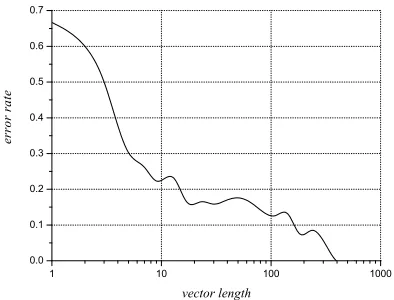
Figure 2: Error Rate vs. Vector Length (smoothed), on CE Collection, 5000 Dimensions byχ2
and the wrongly classified documents are separately investigated, they both yield a nearly lognormal dis-tribution.
Also in Figure 1, wrongly classified documents shows a relatively large proportion at low dimen-sionalities. Figure 2 demonstrates this with more clarity. Thus the hypothesis formed in Section 1 is confirmed: there is a strong correlation between the sparseness degree and the categorization error rate.
Therefore, it is quite straightforward a thought to measure the “sparseness of a term subset” (or more precisely, the exhaustivity) by the corresponding av-erage vector length(AVL) of all documents.4 In the
4Due to the lognormal distribution of vector length, it seems
more plausible to average the logarithmic vector length. How-ever, for a fixed number of documents ,log
P
|dj|
|D| should hold a nearly fixed ratio to
P
log|dj|
[image:3.612.328.525.256.406.2]remainder of this paper, (log) AVL is an important metric used to assess and control the sparseness of a term subset.
4 Scalable Term Selection (STS)
Since the performance droping down at low dimen-sionalities is attributable to lowAVLs in the previous section, a scalable term selection criterion should automatically accommodate its favor of high cov-erage to different target dimensionalities.
4.1 Measuring Discriminability and Coverage
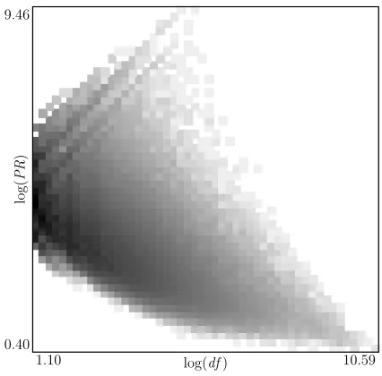
The first step is to separately measure the discrim-inability and the coverage of a term. A basic guide-line is that these two metrics should not be highly (positive) correlated; intuitively, they should have a slight negative correlation. The correlation of the two metrics can be visually estimated by the joint distribution figure. A bunch of term selection met-rics were explored by Forman (2003).df (document frequency) is a straightforward choice to measure coverage. Since df follows the Zipf’s law (inverse power law), log(df) is adopted. High-performing term selection criterion themselves might not be good candidates for the discriminability metric be-cause they take coverage into account. For exam-ple, Figure 3 shows that χ2 is not satisfying. (For readability, the grayness is proportional to the log probability density in Figure 3, Figure 4 and Fig-ure 12.) Relatively,probability ratio(Forman, 2003) is a more straight metric of discriminability.
PR(ti, c) = PP((tti|c+) i|c−) =
df(ti, c+)/df(c+) df(ti, c−)/df(c−)
It is a symmetric ratio, so log(PR) is likely to be more appropriate. For multi-class categorization, a global value can be assessed by PRmax(ti) =
maxcPR(ti, c), like χ2
max for χ2 (Yang and
Ped-ersen, 1997; Rogati and Yang, 2002; Sebastiani, 2002); for brief, PR denotesPRmax hereafter. The
[image:4.612.327.532.59.258.2]joint distribution oflog(PR)andlog(df)is shown in Figure 12. We can see that the distribution is quite even and they have a slight negative correlation.
4.2 Combined Criterion
Now we have the two metrics:log(PR)for discrim-inability andlog(df)for coverage, and a parametric
log(df) χ2
1.10 10.59
1.7 42033.0
Figure 3:¡log(df), χ2¢Distribution, on CE
log(df)
lo
g(
P
R
)
1.10 10.59
[image:4.612.319.532.294.504.2]0.40 9.46
Figure 4:(log(df),log(PR))Distribution, on CE
term selection criterion comes forth:
ζ(ti;λ) =
µ
λ
log(PR(ti))+
1−λ
log(df(ti))
¶−1
of the expected dimensionality (k):
λ∗(k) = arg max
λ
F1(Sk(λ))
in which the term subsetSk(λ) ∈ T is selected by ζ(◦;λ),|Sk|= k, andF1 is the default evaluation criterion. Naturally, this optimalλleads to a corre-sponding optimalAVL:
AVL∗(k)←→λ∗(k)
For a concrete implementation, we should have an (empirical) function to estimateλ∗ orAVL∗:
AVL◦(k)=. AVL∗(k)
In the next section, the values ofAVL∗(as well asλ∗)
for somek-s are figured out by experimental search; then an empirical formula,AVL◦(k), comes forth. It
is interesting and inspiring that by adding the “cor-pus AVL” as a parameter this formula is universal for different document collections, which makes the whole idea valuable.
5 Experiments and Implementation
5.1 Experiments
The expected dimensionalities (k) chosen for exper-imentation are
CE: 500, 1000, 2000, 4000, . . . , 32000, 64000; 20NG: 500, 1000, 2000, . . . , 16000, 30220.5
For a given document collection and a given target dimensionality, there is a correspondingAVLfor aλ, and vice versa (for the possible value range ofAVL). According to the observations in Section 5.2, AVL other thanλis the direct concern because it is more intrinsic, butλis the one that can be tuned directly. So, in the experiments, we varyAVLby tuningλto produce it, which means to calculateλ(AVL).
AVL(λ) is a monotone function and fast to cal-culate. For a given AVL, the corresponding λcan be quickly found by a Newton iteration in [0,1]. In fact, AVL(λ) is not a continuous function, so λ is only tuned to get an acceptable match, e.g. within
±0.1.
5STS is tested to the wholeT on 20NG but not on CE,
be-cause (i)TCEis too large and time consuming for training and testing, and (ii)χ2 was previously tested on largerkand the performance (F1) is not stable whilek >64000.
For each k, by the above way of fitting λ, we manually adjust AVL (only in integers) until F1(Sk(λ(AVL))) peaks. By this way, Figure 5–11 are manually tuned best-performing results as obser-vations for figuring out the empirical formulas.
Figure 5 shows theF1 peaks at different dimen-sionalities. Comparing to χ2, STS has a consid-erable potential superiority at low dimensionalities. The corresponding values ofAVL∗are shown in
Fig-ure 6, along with theAVLs ofχ2-selected term sub-sets. The dotted lines show the trend ofAVL∗; at the overall dimensionality,|TCE|= 1067717, they have
the sameAVL = 898.5. We can see thatlog(AVL∗)
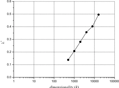
is almost proportional to log(k) when k is not too large. The corresponding values ofλ∗ are shown in
Figure 7; the relation is nearly linear betweenλ∗and
log(k).
Now it is necessary to explain why an empirical AVL◦(k) derived from the straight line in Figure 6
can be used instead of AVL∗(k) in practice. One important but not plotted property is that the per-formance of STS is not very sensitive to a small value change of AVL. For instance, at k = 4000, AVL∗ = 120 and the F1 peak is 85.8824%, and for AVL = 110and130 the corresponding F1 are 85.8683% and 85.6583%; at the same k, the F1 ofχ2 selection is 82.3950%. This characteristic of STS guarantee that the empiricalAVL◦(k)has a very
close performance to AVL∗(k); due to the limited space, the performance curve of AVL◦(k) will not be plotted in Section 5.2.
Same experiments are done on 20NG and the re-sults are shown in Figure 8, Figure 9 and Figure 10. The performance improvements is not as signifi-cant as on the CE collection; this will be discussed in Section 6.2. The conspicuous relations between AVL∗,λ∗andkremain the same.
5.2 Algorithm Completion
In Figure 6 and Figure 9, the ratios oflog(AVL∗(k))
tolog(k) are not the same on CE and 20NG. Tak-ing into account thecorpus AVL(theAVLproduced by the whole term set): AVLTCE = 898.5286 and
AVLT20NG = 82.1605, we guess
log(AVL∗(k))
log(AVLT) is
100 1000 10000 100000 60
65 70 75 80 85 90
F
1
(
%
)
dimensionality (k)
2
[image:6.612.321.530.70.232.2]STS
Figure 5: Performance Comparison, on CE
1 10 100 1000 10000 100000 1000000 1
10 100 1000
2
STS
A
V
L
*
[image:6.612.81.292.72.234.2]dimensionality (k)
Figure 6:AVLComparison, on CE
1 10 100 1000 10000 100000 1000000 0.00
0.02 0.04 0.06 0.08 0.10 0.12
dimensionality (k)
Figure 7: Optimal Weights oflog(PR), on CE
100 1000 10000 100000
72 74 76 78 80 82 84 86
2
STS
F
1
(
%
)
[image:6.612.322.533.294.448.2]dimensionality (k)
Figure 8: Performance Comparison, on 20NG
1 10 100 1000 10000 100000
1 10 100
2
STS
A
V
L
*
dimensionality (k)
Figure 9:AVLComparison, on 20NG
1 10 100 1000 10000 100000
0.0 0.1 0.2 0.3 0.4 0.5 0.6
dimensionality (k)
[image:6.612.81.290.297.451.2] [image:6.612.321.530.511.667.2] [image:6.612.79.289.513.667.2]1 10 100 1000 10000 100000 1000000 0.0
0.2 0.4 0.6 0.8 1.0
l
o
g
(
A
V
L
*
(
k
)
)
/
l
o
g
(
A
V
L
T
)
dimensionality (k)
[image:7.612.80.290.58.217.2]CE 20NG
Figure 11: log(log(AVLAVL∗(k))
T) , on Both CE and 20NG
contains some discussion on this.
From the figure, we get the value of this ratio (the base oflogis set toe):
γ = log(AVL∗(k))/log(AVLT)
log(k) ∼= 0.085
which should be a universal constant for all text cat-egorization tasks.
So the empirical estimation of AVL∗(k) is given by
AVL◦(k) = exp(γlog(AVLT)·log(k)) = AVLTγlog(k)
and the final STS criterion is
ζ(ti, k) = ζ(ti;λ(AVL◦(k))) = ζ(ti;λ(AVLTγlog(k)))
in whichλ(◦) can be calculated as in Section 5.1. The target dimensionality,k, is involved as a param-eter, so the approach is namedscalableterm selec-tion. As stated in Section 5.1,AVL◦(k) has a very
close performance to AVL∗(k)and its performance is not plotted here.
6 Further Observation and Discussion
6.1 Comparing the Selected Subsets
An investigation shows that for a quite large range of λ, term rankings by ζ(ti;λ) and χ2(t
i) have a strong correlation (theSpearman’s rank correlation coefficient is bigger than 0.999). In order to
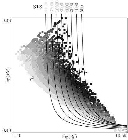
com-log(df)
lo
g(
P
R
)
1.10 10.59
0.40 9.46
50
0
10
00
20
00
40
00
80
00
16
00
0
32
00
0
64
00
0
STS
[image:7.612.318.532.61.296.2]χ2
Figure 12: Selection Area Comparison of STS and χ2on Various Dimensionalities, on CE
log(df)
lo
g
(
P
R
)
1.10 9.14
0.11 8.04
50
0
10
00
20
00
40
00
80
00
16
00
0
STS
[image:7.612.321.532.351.581.2]χ2
Figure 13: Selection Area Comparison of STS and χ2on Various Dimensionalities, on 20NG
dimension-alities, the selection areas of STS are represented by boundary lines, and the selection areas ofχ2are rep-resented by different grayness.
In Figure 12, STS shows its superiority at low di-mensionalities by more emphasis on the coverage of terms. In Figure 13, STS shows its superior-ity at high dimensionalities by more emphasis on the discriminability of terms; lower coverage yields smaller index size and lower computational cost. At any dimensionality, STS yields a relatively fixed bound for either discriminability or coverage, other than a compromise between them likeχ2; this is at-tributable to the harmonic averaging.
6.2 Adaptability of STS
There are actually two kinds of sparseness in a (vec-torized) document collection:
collection sparseness: the high-dimensional learn-ing space contains few trainlearn-ing samples; document sparseness: a document vector has few
nonzero dimensions.
In this study, only the document sparseness is inves-tigated. The collection sparseness might be a back-room factor influencing the actual performance on different document collections. This might explain why the explicit characteristics of STS are not the same on CE to 20NG: (comparing withχ2, see Fig-ure 5, FigFig-ure 6, FigFig-ure 8 and FigFig-ure 9)
CE. The significantF1 improvements at low di-mensionalities sacrifice the short of AVL. In some learning process implementations, it is AVL other than k that determines the computational cost; in many other cases, k is the determinant. Further more, possible post-processing, like matrix factor-ization, might benefit from a lowk.
20NG. TheF1 improvements at low
dimension-alities is not quite significant, but AVL remains a lower level. For higherk, there is less difference in F1, but the smallerAVL yield lower computational cost thanχ2.
Nevertheless, STS shows a stable behavior for various dimensionalities and quite different docu-ment collections. The existence of the universal constant γ empowers it to be adaptive and practi-cal. As shown in Figure 11, STS draws the rela-tivelogAVL∗(k)to the same straight line,γlog(k),
for different document collections. This might means that therelative AVL is an intrinsic demand
for the term subset sizek.
7 Conclusion
In this paper, Scalable Term Selection (STS) is pro-posed and suppro-posed to be more adaptive than tra-ditional high-performing criteria, viz. χ2,IG,BNS, etc. The basic idea of STS is to separately measure discriminability and coverage, and adjust the relative importance between them to produce a optimal term subset of a given size. Empirically, the constant re-lation between target dimensionality and the optimal relative average vector length is found, which turned the idea into implementation.
STS showed considerable adaptivity and stability for various dimensionalities and quite different doc-ument collections. The categorization accuracy in-creasing at low dimensionalities and the computa-tional cost decreasing at high dimensionalities were observed.
Some observations are notable: the loglinear rela-tion between optimal average vector length (AVL∗) and dimensionality (k), the semi-loglinear relation between weight λand dimensionality, and the uni-versal constantγ. For a future work, STS needs to be conducted on more document collections to check if γis really universal.
In addition, there could be other implementations of the general STS idea, via other metrics of discrim-inability and coverage, other weighted combination forms, or other term subset evaluations.
Acknowledgement
The research is supported by the National Natural Science Foundation of China under grant number 60573187, 60621062 and 60520130299.
References
Janez Brank, Marko Grobelnik, Nataˇsa
Milic-Fraylingand, and Dunjia Mladenic. 2002. Interaction of feature selection methods and linear
classifica-tion models. Workshop on Text Learning held at
ICML-2002.
Chih-Chung Chang and Chih-Jen Lin, 2001. LIBSVM: a
George Forman. 2003. An extensive empirical study of feature selection metrics for text classification. Jour-nal of Machine Learning Research, 3:1289–1305.
Evgeniy Gabrilovich and Shaul Markovitch. 2004. Text categorization with many redundant features: using aggressive feature selection to make svms competitive
with c4.5. InICML ’04: Proceedings of the
twenty-first international conference on Machine learning, page 41, New York, NY, USA. ACM Press.
Isabelle Guyon and Andr´e Elisseeff. 2003. An intro-duction to variable and feature selection. Journal of Machine Learning Research, 3:1157–1182.
Thorsten Joachims. 1998. Text categorization with sup-port vector machines: learning with many relevant
fea-tures. In Proceedings of ECML ’98, number 1398,
pages 137–142. Springer Verlag, Heidelberg, DE.
Jingyang Li, Maosong Sun, and Xian Zhang. 2006. A comparison and semi-quantitative analysis of words and character-bigrams as features in chinese text
cat-egorization. In Proceedings of COLING-ACL ’06,
pages 545–552. Association for Computational Lin-guistics, July.
Michael Mitzenmacher. 2003. A brief history of genera-tive models for power law and lognormal distributions.
Internet Mathematics, 1:226–251.
Monica Rogati and Yiming Yang. 2002.
High-performing feature selection for text classification. In Proceedings of CIKM ’02, pages 659–661. ACM Press.
Fabrizio Sebastiani. 2002. Machine learning in
auto-mated text categorization. ACM Computing Surveys
(CSUR), 34(1):1–47.
Yiming Yang and Christopher G. Chute. 1994. An
example-based mapping method for text
categoriza-tion and retrieval. ACM Transactions on Information
Systems (TOIS), 12(3):252–277.
Yiming Yang and Jan O. Pedersen. 1997. A compara-tive study on feature selection in text categorization.
In Douglas H. Fisher, editor, Proceedings of
ICML-97, 14th International Conference on Machine
Learn-ing, pages 412–420, Nashville, US. Morgan