Assessing a Sparse Distributed Memory Using Different Encoding Methods

Assessing a Sparse Distributed Memory

Using Different Encoding Methods

Mateus Mendes

, A. Paulo Coimbra

, and Manuel Cris´

ostomo

Abstract—A Sparse Distributed Memory (SDM) is a kind of associative memory suitable to work with high-dimensional vectors of random data. This mem-ory model is attractive for Robotics and Artificial In-telligence, for it is able to mimic many characteristics of the human long-term memory. However, sensorial data is not always random: most of the times it is based on the Natural Binary Code (NBC) and tends to cluster around some specific points. This means that the SDM performs poorer than expected. As part of an ongoing project, in which we intend to navigate a robot using a sparse distributed memory to store sequences of sensorial information, we tested different methods of encoding the data. Some meth-ods perform better than others, though some may fade particular characteristics present in the original SDM model.

Keywords: SDM, Sparse Distributed Memory, Data Encoding, Robotics

1

Introduction

The Sparse Distributed Memory model was proposed for the first time in the 1980s, by Pentti Kanerva [1]. Kan-erva figured out that such a memory model, based on the use of high dimensional binary vectors, can exhibit some properties similar to those of the human cerebellum. Phenomenons such as “knowing that one knows”, dealing with incomplete or corrupt data and storing events in se-quence and reliving them later, can be mimiced in a nat-ural way. The properties of the SDM are those of a high dimensional binary space, as thoroughly demonstrated in [1]. The author analyses in detail the properties of a model working with 1000-bit vectors, or dimensionality

n= 1000. It should be tolerant to noisy data or incom-plete data, implement one-shot learning and “natural” forgetting, as well as be suitable to work with sequences of events.

In our case, a SDM is used as the basis to navigate a robot based on a sequence of grabbed images. During a learning stage the robot stores images it can grab, and during the autonomous run it manages to follow the same path by correcting view matching errors which may occur [2, 3]. Kanerva proposes that the SDM must be ideal to store sequences of binary vectors, and J. Bose [4, 5] has extensively described this possibility.

Kanerva demonstrates that the characteristics of the model hold for random binary vectors. However, in many

∗_{ESTGOH - Esc. Sup. Tec. Gest. OH, Instituto Polit.}

Coim-bra, Portugal. E-mail: mmendes@estgoh.ipc.pt.

†_{ISR - Institute of Systems and Robotics, Dept. of Electrical}

and Computer Engineering, University of Coimbra, Portugal. E-mail:{acoimbra,mcris}@deec.uc.pt.

Figure 1: One SDM model.

circumstances data are not random, but biased towards given points. Rao and Fuentes [6] already mention this problem, although not a solution. In the case of images, for instance, completely black or white images are not common. Many authors minimise this problem by adjust-ing the memory’s structure, so that it has more memory locations in points where they are needed [7, 8, 9], or use different addressing methods [7, 9]. But this only solves part of the problem, and in some cases may even fade some properties of the model.

We tested different methods of encoding the images and navigation data stored into the SDM, including: Natu-ral Binary Code (NBC), NBC with a different sorting of the numbers, integer values and a sum-code. The per-formance of the memory was assessed for each of these methods, and the results are shown.

Sections 2 and 3 briefly describe the SDM and the ex-perimental platform used. Section 4 explains the en-coding problem in more detail and presents two widely used models of the SDM. Section 5 explains two novel ap-proaches, and section 6 presents and discusses our tests and results. Finally, in section 7 we draw some conclu-sions and point out some possible future work.

2

Sparse Distributed Memories

One possible implementation of a SDM is as shown in Figure 1. It comprises two main arrays: one stores the locations’ addresses (left), the other contains the data (right). In the auto-associative version of the model, as used here, the same vector can be used simultaneously as address and data, so that only one array is necessary. Kanerva proposes that there are much less addresses than the addressable space. The actually existing locations are called “hard locations”. This is both a practical con-straint and a requirement of the theory. On one hand, it’s not feasible to work with, e.g., 21000

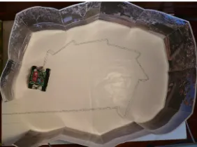
Figure 2: Robot and experimental platform.

In a traditional computer memory one input address shall only activate one memory location, which can then be read or written. In an SDM, however, addressing is done based on the use of an access circle: all the hard locations within a given radius are activated for reading or for writ-ing. Kanerva proposes the Hamming distance (HD) to compute the set of active locations. The HD is actually the number of bits in which two binary numbers differ:

dh(x, y) = P_i(|xi−yi|). In the example (Fig. 1), the

radius is set to 3 bits, and the input address is00110011_.

Therefore, the first and third hard locations are activated, for they differ from the input address, respectively, 2 and 3 bits. The second and fourth hard locations differ 7 and 4 bits and are, therefore, out of the access circle.

The “hard locations” don’t actually store the data as it is input to the memory: they are composed of bit coun-ters. During a write operation, the bit counters of the selected hard locations are incremented to store ones and decremented to store zeros. During a read operation, the active bit counters are summed columnwise and averaged. If the average of the sum for a given bit is above a set threshold, then it shall be one, otherwise it shall be zero.

3

Experimental setup

Some experiments were carried out using a small robot, which was taught a path and was expected to follow it later. The experimental platform used is a small robot with tank-style treads and differential drive, as shown in Fig. 2 and described in more detail in [10].

For navigation using a sequence of images, we follow Y. Matsumoto’s proposal [2]. This requires a super-vised learning stage, during which the robot is manually guided, and a posterior autonomous navigation stage. During the learning stage the robot captures views of the surrounding environment, as well as some additional data, such as odometric information. During the au-tonomous run, the robot captures images of the environ-ment and uses them to localise itself and follow known paths, based on its previously acquired knowledge. This technique has been extensively described in [2, 3]. The SDM is used to store those sequences of images and image data. Input and output vectors consist of arrays of bytes, meaning that each individual value must fit in the range [0, 255]. Every individual value is, therefore, suitable to store the graylevel value of an image pixel or an 8-bit integer.

The composition of the input vectors is:

xi=< imi, seq id, i, timestamp, motion > (1)

imiis imagei. seq idis an auto-incremented 4-byte

inte-ger, unique for each sequence. It is used to identify which sequence the vector belongs to. iis an auto-incremented 4-byte integer, unique for every vector in the sequence. It is used to quickly identify every image in the sequence.

timestamp is a 4-byte integer, storing Unix timestamp. It is read from the operating system, but not being used so far for navigation purposes. motion is a single byte, identifying the type of movement the robot performed just before capturingimi.

Images of resolution 80x64 are used. Since every pixel is stored as an 8-bit integer, the image alone needs 80×64 = 5120 bytes = 40960 bits. The overhead information comprises 13 additional bytes, meaning the input vector contains 41064 bits.

The memory is used to store vectors as explained, but addressing is done using just the image, not the whole vector. The remainder bits could be set at random, as Kanerva suggests, but it was considered preferable to set up the software so that it is able to calculate similarity between just part of two vectors, ignoring the remain-der bits. This saves computational time and reduces the probability of false positives being detected.

4

Practical problems

The original SDM model, though theoretically sound and attractive, has some problems which one needs to deal with.

One problem is that of placing the hard locations in the address space. Kanerva proposes that they are placed at random when the memory is created, but many au-thors state that’s not the most appropriate option. D. Rogers [8], e.g., evolves the best locations using genetic algorithms. Hely proposes that locations must be created where there is more data to store [9]. Ratitch et al pro-pose the Randomised Reallocation algorithm [7], which is essentially based on the same idea: start with an empty memory and allocate new hard locations when there’s a new datum which cannot be stored in enough existing locations. The new locations are allocated randomly in the neighbourhood of the new datum address. This is the approach used here.

Another big weakness of the original SDM model is that of using bit counters. This results in a low storage rate, which is about 0.1 bits per bit of traditional computer memory, huge consumption of processing power and a big complexity of implementation. To overcome this dif-ficulty we simply dropped the counters and built two different models: one called “bitwise implementation” (BW), and another which uses an arithmetic distance (AD) instead of the HD, called “arithmetic implemen-tation” (AR).

Figure 3: Bitwise SDM, which works with bits but not bit counters.

Figure 4: Arithmetic SDM, which works with byte inte-gers, instead of bit counters.

store one bit, instead of a bit counter, under normal cir-cumstances. For real time operation, this simplification greatly reduces the need for processing power and mem-ory size. Fig. 3 shows this simplified model. Writing is simply to replace the old datum with the new datum. Additionally, since we’re not using bit counters and our data can only be 0 or 1, when reading, the average value of the hard locations can only be a real number in the interval [0,1]. Therefore, the best threshold for bitwise operation is at 0.5.

The arithmetic model is inspired by Ratitch et al’s work [7]. In this variation, the bits are grouped as integers, as shown in Fig. 4. Addressing is done using an arithmetic distance, instead of the HD [3]. Learning is achieved using a reinforcement learning algorithm:

hk_t =hk_t

−1+α·(x k_−hk

t−1), α∈R∧0≤α≤1 (2)

hk

t is the kth number of the hard location, at timet. xk

is the corresponding number in the input vectorxandα

the learning rate.

5

Binary codes and distances

In natural binary code the value of each bit depends on its position. 01 _{is different from} 10_{. This}

characteris-tic means that the HD is not proportional to the binary difference of the numbers.

Table 1 shows the HDs between all the 3-bit binary num-bers. As it shows, this distance is not proportional to the arithmetic distance. The HD sometimes even decreases when the arithmetic difference increases. One example is the case of 001_to 010_{, where the arithmetic distance is}

1 and the HD is 2. And if we compare001 _to 011_{, the}

arithmetic distance increases to 2 and the HD decreases to 1. In total, there are 9 undesirable situations in the

Table 1: Hamming distances for 3-bit numbers.

000 001 010 011 100 101 110 111

000 0 1 1 2 1 2 2 3

001 0 2 1 2 1 3 2

010 0 1 2 3 1 2

011 0 3 2 2 1

100 0 1 1 2

101 0 2 1

110 0 1

111 0

Table 2: Example distances using different metrics.

Pixel value Distance

im_i im_j Arit. Hamming Vanhala

01111111 10000000 1 8 1

11111111 00000000 127 8 1

table, where the HD decreases while it should increase or, at least, maintain its previous value. The problem of this characteristic is that the PGM images are encoded using the Natural Binary Code, which takes advantage of the position of the bits to represent different values. But the HD does not consider positional values. The performance of the SDM, therefore, might be affected because of these different criteria being used to encode the information and to process it inside the memory.

These characteristics of the NBC and the HD may be ne-glectable when operating with random data, but in the specific problem of storing and retrieving graylevel im-ages, they may pose serious problems. Suppose, for in-stance, two different copies, imi and imj, of the same

image. Let’s assume a given pixel P has graylevel 127 (01111111_{) in imi. But due to noise, P has graylevel}

128 (10000000_{) inimj. Although the value isalmost the}

same, the hamming distance between the value of P in each image is the maximum it can be—8 bits.

Vanhala et al. [12] use an approach that consists in us-ing only the most significant bit of each byte. This still relies on the use of the NBC and is more robust to noise. However, this approach should work as a very rough fil-ter, which maps the domain [0, 255] onto a smaller do-main [0, 1], where only binary images can be represented. While effective reducing noise, which Vanhala reports to be the primary goal, this mapping is not the wisest so-lution to the original problem we’re discussing. To ef-fectively store graylevel images in the SDM, we need a better binary code. For example, one in which the num-ber of ones is proportional to the graylevel value of the pixel. In this aspect, Vanhala’s approach should not per-form well. The distance from a black pixel (00000000₎

to a white pixel (11111111_{), for instance, is the same as}

between two mid-range pixels which are almost the same, as in the example ofimiandimj described above. Table

2 summarises some example distances.

5.1

Gray code

Table 3: 3-bit natural binary and Gray codes.

Natural BC Gray code

000 000

001 001

010 011

011 010

100 110

101 111

110 101

111 100

Table 4: Hamming distances for 3-bit Gray Code.

000 001 011 010 110 111 101 100

000 0 1 2 1 2 3 2 1

001 0 1 2 3 2 1 2

011 0 1 2 1 2 3

010 0 1 2 3 2

110 0 1 2 1

111 0 1 2

101 0 1

100 0

one.

The GC, as summarised in Table 3, though, also exhibits an undesirable characteristic: it is circular, so that the last number only differs one single bit from the first one. In the case of image processing, in the worst case this means that a black image isalmosta white image. There-fore, the GC is not the ideal one to encode information to store in an SDM. Table 4 shows all the HDs for a 3-bit GC. As happens in NBC, there are also undesirable tran-sitions. For example, the HD between000_and 011_{is 2,}

and the HD between 000_and 010 _{is 1, while the}

arith-metic distances are, respectively, 2 and 3. In conclusion, while the GC might solve a very specific problem, it is not a general solution in this case.

5.2

Sorting the bytes

Another approach is simply to sort the bytes in a more convenient way, so that the HD becomes proportional to the arithmetic distance—or, at least, does not exhibit so many undesirable transitions.

This sorting can be accomplished by trying different per-mutations of the numbers and computing the matrix of hamming distances. For 3-bit numbers, there are 8 dif-ferent numbers and 8! = 40,320 permutations. This can easily be computed using a modern personal computer, in a reasonable amount of time. After an exhaustive search, different sortings are found, but none of them ideal. Table 5 shows a different sorting, better than the NBC shown in Table 1. This code shows only 7 undesirable transi-tions, while the NBC contains 9. Therefore, it should perform better with the SDM, but not outstanding. It should also be mentioned that there are several sortings with similar performance. There are 2,783 other sortings that also have 7 undesirable transitions. The one shown is the first that our software found.

While permutations of 8 numbers are quick to compute, permutations of 256 numbers generate 256!∼= 8.58×10506

sortings, which is computationally very expensive. How-ever, there are several sortings that should exhibit similar

Table 5: Hamming distances for 3-bit numbers.

000 001 010 100 101 111 011 110

000 0 1 1 1 2 3 2 2

001 0 2 2 1 2 1 3

010 0 2 3 2 1 1

100 0 1 2 3 1

101 0 1 2 2

111 0 1 1

011 0 2

110 0

performance. The sorting shown in Table 5 was found after 35 out of 40,320 permutations. In the case of 16 numbers (4 bits), a sorting with just 36 undesirable tran-sitions, the minimum possible, is found just after 12 per-mutations. Therefore, it seems reasonable to assume that after just a few permutations it is possible to find one sorting with minimum undesirable transitions, or very close to it. This assumption also makes some sense con-sidering that the number of ones in one binary word is strongly correlated with its numerical value. Big num-bers tend to have more ones and small numnum-bers tend to have less.

The natural binary code shows 18,244 undesirable tran-sitions. Picking 5,000 random sortings, we found an av-erage number of undesirable transitions that was 25,295. Even after several days of computation, our software was not able to randomly find a better sorting. As described above, this makes some sense, considering the dimension of the search space and also that the NBC is partially sorted.

A different approach was also tried, which consisted in testing different permutations, starting from the most significant numbers (these contain more ones). After 57,253,888 permutations our software found one sorting with just 18,050 undesirable transitions1

.

It is not clear if there is a better sorting, but up to 681,400,000 permutations our software was not able to spot a better one. The numbers 244 to 255 have been tested for theirbest position, but the other ones haven’t. Another question may be asked: shall the performance of all the sortings which exhibit the same number of unde-sirable transitions be similar? The answer might depend on the particular domain. If the data are uniformely dis-tributed, then all the sortings shall exhibit a similar per-formance. But if the occurrence of data is more probable at a particular subrange, then the sorting with less unde-sirable transitions in that subrange is expected to exhibit the best performance. In our case, we are looking for the best code to compute the similarity between images. If those images are equalised, then the distribution of all the brightness values is such that all the values are approximately equally probable. This means that it is irrelevant which sorting is chosen, among those with the same number of undesirable transitions.

1_{0 1 ... 242 243 245 249 253 252 255 254 246 250 248 244 247}

Table 6: Code to represent 5 graylevels.

0 0000

1 0001

2 0011

3 0111

4 1111

5.3

Reducing graylevels

As written previously, using 256 graylevels it’s not pos-sible to find a suitable binary code with minimum un-desirable transitions, so that one can take advantage of the representativity of the NBC and the properties of the SDM. The only way to avoid undesirable transitions at all is to reduce the number of different graylevels to the number of bits + 1 and use a kind of sum-code. There-fore, using 4 bits we can only use 5 different graylevels, as shown in Table 6. Using 8 bits, we can use 9 graylevels and so on. This is the only way to work with a hamming distance that is proportional to the arithmetic distance. The disadvantage of this approach, however, is obvious: either the quality of the image is much poorer, or the dimension of the stored vectors has to be extended to accommodate additional bits.

6

Tests and results

Different tests were performed in order to assess the be-haviour of the system using each of the approaches de-scribed in the previous sections. The results were ob-tained using a sequence of 55 images. The images were equalised, and the memory was loaded with a single copy of each.

6.1

Results

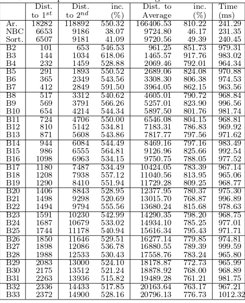
Table 7 shows the average of 30 operations. The tests were performed using the arithmetic distance; using the NBC and the hamming distance (8 bits, 256 graylevels, represented using the natural binary code); using the the hamming distance and a partially optimised sorting of the bytes, as described in section 5.2; and bitwise modes in which the graylevels were reduced to the number of bits + 1, as described in section 5.3. We tested using from 1 to 32 bits, which means from 2 to 33 graylevels, in order to experimentally get a better insight on how the number of bits and graylevels might influence the performance of the system.

The table shows the distance (error in similarity) from the input image to the closest image in the SDM; the distance to the second closest image; and the average of the distances to all the images. It also shows, in percent-age, the increase from the closest prediction to the second and to the average—this is a measure of howsuccessful

the memory is in separating the desired datum from the pool of information in the SDM. We also show the av-erage processing time for each method. Processing time is only the memory prediction time, it does not include the image capture and transmission times. The clock is started as soon as the command is issued to the SDM and stopped as soon as the prediction result is returned.

Table 7: Experimental results using different metrics.

Dist. Dist. inc. Dist. to inc. Time to 1st _{to 2}nd _{(%) Average (%) (ms)}

Ar. 18282 118892 550.32 166406.53 810.22 241.29 NBC 6653 9186 38.07 9724.80 46.17 231.35 Sort. 6507 9181 41.09 9720.56 49.39 240.45 B2 101 653 546.53 961.25 851.73 979.31 B3 144 1034 618.06 1465.57 917.76 983.02 B4 232 1459 528.88 2069.46 792.01 964.34 B5 291 1893 550.52 2689.06 824.08 970.88 B6 365 2349 543.56 3308.30 806.38 974.53 B7 412 2849 591.50 3964.05 862.15 963.56 B8 517 3312 540.62 4605.01 790.72 968.84 B9 569 3791 566.26 5257.01 823.90 996.56 B10 654 4214 544.34 5897.50 801.76 981.74 B11 724 4706 550.00 6546.08 804.15 968.81 B12 810 5142 534.81 7183.31 786.83 969.92 B13 871 5608 543.86 7817.77 797.56 971.62 B14 944 6084 544.49 8469.16 797.16 983.49 B15 986 6555 564.81 9126.96 825.66 992.54 B16 1098 6963 534.15 9750.75 788.05 977.52 B17 1180 7487 534.49 10424.05 783.39 967.14 B18 1208 7938 557.12 11040.56 813.95 965.06 B19 1290 8410 551.94 11729.28 809.25 968.77 B20 1406 8843 528.95 12377.95 780.37 975.30 B21 1498 9298 520.69 13015.70 768.87 996.89 B22 1494 9794 555.56 13680.24 815.68 978.63 B23 1591 10230 542.99 14290.35 798.20 968.75 B24 1687 10679 533.02 14934.10 785.25 977.01 B25 1744 11178 540.94 15616.34 795.43 971.71 B26 1850 11646 529.51 16277.14 779.85 974.81 B27 1898 12086 536.78 16880.55 789.39 999.59 B28 1988 12533 530.43 17558.76 783.24 965.80 B29 2083 13000 524.10 18178.87 772.73 965.99 B30 2175 13512 521.24 18878.92 768.00 968.89 B31 2263 13936 515.82 19489.28 761.21 981.75 B32 2336 14433 517.85 20163.64 763.17 967.21 B33 2372 14900 528.16 20796.13 776.73 1012.32

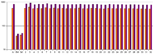
For clarity, chart 5 shows, using a logarithmic scale, the increments of the distance from the closest image to the second closest one (lighter colour) and to the average of all the images (darker colour).

6.2

Analysis of the results

It can be confirmed that the bitwise mode using the NBC seems to be remarkably worse than the other methods, which seem to show similar results. Sorting the bytes results in a small, but not significant, improvement. An-other interesting point is that the number of graylevels seems to have little impact on the selectivity of the image, for images of this size and resolution.

The processing time exhibits a great variation, for the tests were run on a computer using Linux (OpenSuSE 10.2), abest effort operating system. Even with the num-ber of processes running down to the minimum, there were very disparate processing times. For better preci-sion and real time operation, a real time operating system would be recommended.

Figure 5: Error increments. Light colour: to the second best image. Darker: to the average.

memory access time. A more efficient approach would be to make the conversion as soon as the images were grabbed from the camera. This is undesirable in our case, though, as we’re also testing other approaches.

As for the other approaches using different graylevels, the processing times are all similar and about 4 times larger than the time of processing one image using the arithmetic mode. The reason for this is that, again, an indexed table is used to address the binary code used. And in this case there’s the additional workload of pro-cessing the conversion into the desired number of gray values. In a production system, obviously, the conversion would only need to be done once, just as the images were grabbed from the camera.

7

Conclusions and future work

We described various tests to assess the performance of a Sparse Distributed Memory with different methods of encoding the data and computing the distance between two memory items.

In the original SDM model Kanerva proposes that the hamming distance be used to compute the similarity be-tween two memory items. Unfortunately, this method exhibits a poor performance if the data are not random. The NBC with the hamming distance shows the worst performance. By sorting some bytes the performance is slightly improved. If the bits are grouped as bytes and an arithmetic distance is used, the memory shows an excel-lent performance, but this can fade some characteristics of the original model, which is based on the properties of a binary space. If the number of graylevels is reduced and a sum-code is used, the performance is close to that of the arithmetic mode and the characteristics of the memory must still hold..

Although our work was performed using images as data, our results should still be valid for all non-random data, as is usually the case of robotic sensorial data.

Future work includes the study of the impact of using different encoding methods on the performance of the SDM itself, in order to infer which characteristics shall still hold or fade.

References

[1] Pentti Kanerva. Sparse Distributed Memory. MIT Press, Cambridge, 1988.

[2] Yoshio Matsumoto, Masayuki Inaba, and Hirochika Inoue. View-based approach to robot navigation. In

Proc. of 2000 IEEE/RSJ International Conference on Intelligent Robots and Systems (IROS 2000), 2000.

[3] Mateus Mendes, Manuel Cris´ostomo, and A. Paulo Coimbra. Robot navigation using a sparse dis-tributed memory. In Proc. of the 2008 IEEE In-ternational Conference on Robotics and Automation, Pasadena, California, USA, May 2008.

[4] Joy Bose. A scalable sparse distributed neural mem-ory model. Master’s thesis, University of ester, Faculty of Science and Engineering, Manch-ester, UK, 2003.

[5] Joy Bose, Steve B. Furber, and Jonathan L. Shapiro. A spiking neural sparse distributed memory im-plementation for learning and predicting temporal sequences. In International Conference on Artifi-cial Neural Networks (ICANN), Warsaw, Poland, September 2005.

[6] Rajesh P.N. Rao and Olac Fuentes. Hierarchical learning of navigational behaviors in an autonomous robot using a predictive sparse distributed memory.

Machine Learning, 31(1-3):87–113, April 1998. [7] Bohdana Ratitch and Doina Precup. Sparse

dis-tributed memories for on-line value-based reinforce-ment learning. InECML, 2004.

[8] David Rogers. Predicting weather using a genetic memory: A combination of kanerva’s sparse dis-tributed memory with holland’s genetic algorithms. InNIPS, 1989.

[9] Tim A. Hely, David J. Willshaw, and Gillian M. Hayes. A new approach to kanerva’s sparse dis-tributed memories. IEEE Transactions on Neural Networks, 1999.

[10] Mateus Mendes, A. Paulo Coimbra, and Manuel Cris´ostomo. AI and memory: Studies towards equip-ping a robot with a sparse distributed memory. In Proc. of the IEEE International Conference on Robotics and Biomimetics, Sanya, China, Dec. 2007. [11] Stephen B. Furber, John Bainbridge, J. Mike Cump-stey, and Steve Temple. Sparse distributed memory using n-of-m codes. Neural Networks, 17(10):1437– 1451, 2004.