Abstract—With new services provided by airlines and travel agencies passengers gained more flexibility, but also their visibility for airports and airlines was decreased. We describe the profiling component of a movement forecast system to increase passenger transparency. Therefore we present three approaches to learning classifiers and how they can be used for passenger classification. It is shown how the choice of attributes considered in classification influences classifier performance. This is used as a comparison criterion for learning algorithms.
Index Terms—accuracy estimation, comparing classifiers, feature subset selection, passenger classification
I. INTRODUCTION
The constantly increasing number of air traffic passengers over the last years requires either the expansion of existing infrastructures like terminal buildings or the construction of new airports.
Modern terminal buildings can be designed with a layout that allows different streams of passengers being separated from each other in compliance with regulations for passenger flows like domestic, Schengen, international, arriving, departure, or transit. However, existing terminals are restricted in their infrastructure and have to find a possible integration of regulations and control for the passenger flows. In addition, passengers get lost, and suffer from raised stress levels. They might cause the delay of flights due to different passenger handling philosophies – from past time periods – as well as regulation by authorities varying from country to country.
Airlines and travel agencies continuously improve their extensive services to manage and simplify the passenger’s travel with respect to flexibility. For example, passengers can check in at home to avoid long queuing lines at the airport – if they travel without check-in luggage (common for domestic or short range business traveler). Unfortunately, these passengers are not visible for the airlines until the moment where they pass the departure gate. Note that passenger pass through several security checks and border controls without any notification to the airlines.
In this publication, we discuss some aspects of the
Manuscript received December 8, 2008.
S. Richter is with EADS Innovation Works of the EADS Deutschland GmbH, 21129 Hamburg, Germany (phone: +49-40-74381510; fax: +49-40-74381517; e-mail: [email protected])
C. Ortmann is with EADS Innovation Works of the EADS Deutschland GmbH, 21129 Hamburg, Germany (e-mail: [email protected])
T. Reiners is with Institute of Information Systems of the University of Hamburg, Germany (e-mail: [email protected])
methodology for a system to support airlines and airports with respect to the transparency of passengers, i.e. to detect late- or no-show passengers as early as possible.
II. SYSTEM OVERVIEW
We developed an airport movement forecast system to detect late- or no-show passengers in an early stage and to predict the routes of passengers – based on their characteristics – already being present at the airport; with calculations being done in or close to real-time. In addition, the system can provide optimized routes for the single passenger to guide him smoothly and without stress throughout the terminal. That is, passengers can ask for guidance to so-called Points of Interests (POI) and the system will determine the (best) route in accordance to feasibility checks. These checks include estimations if the passenger can visit his POIs and still arrive at the gate in time. Furthermore, the system can determine if the POI is out of scope for the passenger, e.g. a domestic traveler cannot access the duty free area. There are other minor checks to assure plausible results of the system but these are not further discussed in this paper. For the system a modular approach is used to provide flexibility for different operating systems and hardware architectures, or a later system optimization being described in Section VII. The modular architecture also supports extensibility, scalability, and refactoring of modules to prevent large or unstructured systems.
All other components are linked to a centralized database system. The database stores third party data like up-to-date passenger data from airlines, travel agencies, and tracking data from the airport and ground handlers. Other components of the overall system are modules dealing with, e.g., communication, calculation, or classification.
In the current development stage, the route calculation module cover the complete route prediction calculation, see [1]. It was planned from the beginning that this is an intermediate step as the prediction of reliable movement information for each passenger had to be improved using more sophisticated algorithms. Nevertheless, the algorithms were chosen in a way that they can later be modified by another system component.
In this paper we introduce passenger classifier, which are used for calculations to forecast the routes according to the specific characteristics of individual passengers.
III. SYSTEM IN- AND OUTPUT
The prediction of routes requires a certain set of passenger attributes that are obtained from third party applications. The results of our calculations can be redistributed to third party
Passenger Classification for an Airport
Movement Forecast System
applications like airline systems to show the passengers’ status per flight or airport to identify bottlenecks on a short term basis, which are not covered by long term resource planning systems [2]. And of course the passengers can get the latest flight information, e.g. gate changes or delays.
A. Input parameters
To predict the route of a passenger the actual position needs to be known. Therefore, the airport terminal is divided into zones to allow localization methods to report the position to our system. Using variable zones makes the whole installation flexible and easily adaptable to the requirements of different airports. Even though the zone size does not have to be limited for the system, several drawbacks are related to the actual zone sizes. In case of very large zones, the prediction of the passenger’s position might not be precise, whereas small zones increase the problem size exponentially and require additional filters to handle irrational passenger movements. Note that the latter reason also explains why no movement vector is required as input, but only the unique identifier of the zone.
Legacy airport systems provide flight related data like departure gate, estimated departure time, possible gate changes, and the flight identifier (also known as flight number).
Finally, individual data of the passenger is used to link the passenger to the right passenger category. These categories can concern age, gender, movement abilities with respect to, e.g., stairs as well as further optional parameters like requested guidance, airline bonus programs, or profession. These optional parameters can be widely extended whereas the classifier should not rely on them and rather work with a minimum set. In case of requested guidance, the chosen POIs are additional parameters to the system.
The privacy of the passenger is mandatory – and even enforced by national laws – so that names or contact details are not used for the calculations, independent of the fact that all additional information about the passenger could improve the output quality of the system.
In this paper, we consider the layout of the airport to be static and, therefore, it is not used as an input parameter. Nevertheless, the system could handle dynamic layouts, which occur, e.g., in case of areas being blocked due to cleaning, special events, or security problems.
B. Output parameters
The overall system can provide a large variety of data and can be used to monitor passenger flows in a live environment, calculate bottlenecks online – e.g. at security check points or border controls – identify crowded airport zones, and distribute the load in the zones more equally in case of guided passengers. The system provides functionality to calculate the time that a passenger needs to reach the gate under all present constraints including optional intermediate POIs. The system also provides detailed route information to the passenger. Depending on the passenger’s guidance settings the route is a forecast (for non-guided person) or an optimal route taking the environmental conditions of the airport into consideration (for guided person).
Stakeholders like airlines and airports are more interested
in the condition of each single passenger. For example, this can indicate if a passenger has still enough time to reach the gate or if someone needs help, or is even going to miss the flight. The advantage of the system is that it can recognize these situations long before even the boarding has begun e.g. due to large queues at border controls or limited movement capabilities. Furthermore, the system gives an indication about what causes the possible delay of the passenger, so that the personnel can act appropriately.
IV. CLASSIFICATION CONSTRAINTS
A. General Constraints
The main purpose of the system is the forecast of a more precise movement route and time for each passenger to reduce the uncertainty of late arrival, which are reasons for flight delays. With the path calculation from [1] and its flexible design, the next step was the investigation of the possibilities, to categorize passengers according to their specific attributes listed in Section III. Some of the parameters had to be derived from non-personal data e.g. the departure time or waiting times at the airport. Nevertheless, the number of attributes per passenger is restricted, mainly for privacy reasons.
Basically, the classification module should take the available data from the data base and link the passenger with a class of behavior attributes to be used in the path calculation. A more sophisticated classification method results in a more reliable forecast for the stakeholders. That is, the estimated walking time of each passenger including the preferred POIs on the route; this could be either shops, restaurants, or other configurations.
The classifiers are constrained by this limited data as well as the uncertain data basis during the training process of the system. Especially, if we intend to allow installation of the system at every airport worldwide without conducting long surveys to build up the data basis. Furthermore, we assume that the behavior of the people is changing periodically throughout the seasons of the year. Section V outlines approaches how the used classification methods cope with these constrains automatically.
B. Training Constraints
Training datasets – where passenger data is being linked to specific target classes – are needed for the learning process of classifiers. The class allocation can only be done in a reliable manner when the passenger is surveyed throughout his time in the airport terminal. This can be achieved e.g. by a tracking system. The tracking data contains the passenger movements and describes the chosen routes of each passenger through the terminal tagged with time stamps to estimate walking times.
classification task is to map unseen passengers to the corresponding classes shown in Fig. 1.
Fig. 1 Classes for different walking speed
The second step is the classification of the passengers’ preferred routes with respect to the characteristics of the visited nodes in the terminal zone network. Here, we have to distinguish the individual preferences of passengers’ preferences – that is the weight towards a specific POI-class – to establish the classes for the routes: Some prefer to visit a restaurant while others use their time for last minute shopping in duty free stores. Note that the exact number of classes depends on the airport infrastructure and the options passengers can choose from.
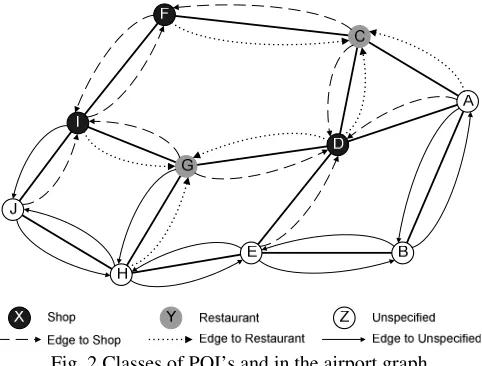
[image:3.595.49.290.449.632.2]The classifier for the routes is given by a graph representation for the airport layout [1]. In this graph, which is also used for the route determination, the destination of the directed edges is equivalent to the corresponding POI-classes of the nodes; see also Fig. 2. Black represents the POI-class shop and grey the POI-class restaurant while the other nodes in this scenario have no specific attributes. All edges towards one node have the same POI-class and color, respectively. In Fig. 2, we assume that node A represents the security checkpoint and node J the departure gate.
Fig. 2 Classes of POI’s and in the airport graph To classify a passenger, its route data is mapped onto the graph. The node type that is visited most on the route from the border security (A) to the gate (J) represents the POI-class for the passenger.
Table I: Path’ along preferred POI’s Passenger Observed path Preference
1 A-C-F-I-J Shops
2 A-C-D-G-H-J Restaurants
3 A-D-E-H-J No preference
Table I shows three examples with different preferences of surveyed passengers. The first one chose a path from the border security (A) to the departure gate (J) passing through one restaurant node (C) and two shop nodes (F, I), so the passenger is classified in the POI-class shop. The second passenger has two restaurants (C, G), one shop (D) and one unspecified (H) on the route and belongs therefore to the POI-class restaurant. The third passenger shows no preferences as the route is going mainly through unspecified nodes. The preference is determined for all passengers.
V. PASSENGER CLASSIFIER
The previous section described how the training data is used to determine the classes for walking speed as well as preferred route (POI-classes). Next, we apply these information to new passengers to acquire their POI-class, which is then added to the attributes of the passengers and used to determine the best walking speed class and, therewith, the time required to arrive at the gate.
In general, learning algorithms can be divided into eager and lazy learners [4]. An eager learner needs a model – being built earlier from a given set of passengers for whom the correct classification is already known – to perform a new classification process on unknown data.
In contrast, a lazy learner only relies on the given dataset in order to assess the classification of a previously unknown passenger. Therefore, no training has to be performed in advance. The nearest neighbor classifier is the only representative of the group of lazy learners we tested [7].
The initial training process of this classifier might be inconvenient if one is installing the system in a new airport, as the system cannot be set operationally right from the beginning.
The following list summarizes possible methods and describes their (dis-)advantages for the classification module of the overall system.
A. Decision Trees
The special nature of the operational environment of the system implies classifiers, which can be used without previous training and allow an immediate adaptation in case of specific configurations. One possibility is a decision tree with predefined but adaptable rules. Fig. 3 shows a decision tree with basic branching rules.
In the decision tree, each node represents an attribute test, while the leaves represent conclusions; in this case they are the class labels. Therefore, each path from the root to a leaf can be interpreted as a decision rule, e.g. each passenger with normal mobility and age between twenty and thirty would be classified as FAST. These rules do not cover all attributes of the passenger, but only the ones for which we expect a significant impact on the decision; e.g. age and mobility. Afterwards, the scale is increased by applying further rules. Note that rules cannot be reduced.
F a s te s t F a s t N o rm a l S lo w S lo w e s t N o rm a l S lo w S lo w e s t N o rm a l S lo w e r S lo w
Fig. 3 A simple decision tree
drops below a predefined threshold, the classifier is adapted with respect to the collected passenger data as follows:
1. First, the classes linked to the leaves of the tree are altered. For each decision rule, the subset of the training dataset – which fulfills this rule – is determined. All objects of the subset have been allocated to the same class by the classifier and, e.g., contain all passengers being of normal mobility and of age between twenty and thirty years. According to the decision tree in Fig. 3, all passengers in this subset would be classified as FAST. Next, the current target class distribution is calculated. If the results indicate a deviation of the major subset class from the predicted one, e.g. the majority of passengers in the subset are observed being SLOW instead of FAST. The class allocation of the leaf is changed to the true class dominating the subset.
2. Afterwards, the tree is expanded similar to the method described in [5]. This is done if a certain amount of objects in a subset are misallocated and a change of the class allocation of the leaf does not result in a better accuracy. A rule based classification method is used on the subset to identify new rules to describe the subset. For example, new rules can split a subset where passengers having a frequent flyer status belong to class FAST, while the others are observed as being SLOW. The tree is expanded for this leaf applying the new rules, i.e. adding an attribute test that separates passengers with and without a frequent flyer status. Two leaves with corresponding class labels are added to the new tree node.
Instead of expanding the tree step by step, another approach uses a full spanning tree with all possible rules based on the given attributes. As before links between the leaves and the classes are based on given data.
Under the assumption that the prerequisites are the same the classification results of both approaches are the same. Also the classification modifications follow the same procedure, but only up to the first step of a new leaf allocation. Despite the advantage that an operational classifier is available where the learning is done while new passengers are classified, decision trees bear the disadvantage that changes in the passengers’ behavior causes trees to become obsolete. A new model has to be built from the beginning. This is especially the case with the incremental tree, as an expansion of certain branches of the tree cannot be undone. Although in
the full tree approach the model could be adapted to changes in the passengers’ behavior, this would be more time consuming than building a new incremental tree, where every leaf of the fully expanded tree needs to be examined.
B. Neural Network
In analogy to the human brain, a neural network consists of interconnected simple neurons (nodes), generally structured in three layers (input, hidden, output). The neurons use activation functions that calculate the input of all (connected) neurons from the previous layer to an output value for the next layer. The activation function is often based on a threshold like the delta function or the sigmoid. To derive arguments for its activation function from it, a linear combination of the inputs of a neuron’s predecessors is formed using certain weights. In this paper, we assume that the layers are fully linked: every node from one layer is linked to all nodes of the following layer. The weights of the links are initialized with random real numbers in the interval [0, 1].
A network consists of an input layer, which is provided with a vector representation of the object to classify, a certain number of hidden layers and an output layer with one unit for each possible class [6]. The passenger classification using neural networks requires an encoding as a vectorxrwith the passengers attributes being mapped to the components xi of
this vector. The activation of the nodes in the input layer is determined by the values of the attributes, whereas we have to distinguish the type of the attributes. In case of interval scaled attributes, the xi is set to the respective value of the attribute.
For a discrete attribute ak with n possible values (aki, i=0,…,
n-1), a segment xl to xm , m-l = n of the vector x r
is used to encode the current value by setting xl+i to 1 and all others in
this segment to 0. Note that the values of the attribute need to be serialized beforehand.
The number of nodes in the output layer of the network equals the number of different classes and is encoded similar to input layer. Therefore, the vector for the classification of passengers from the training set is encoded according to equation (1):
{ }
n{ }
ni i C o o o
o 0,1 , 1, 1,0
1 ∈ = ∀ ∈
∑
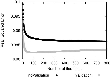
= r r r (1) The network topology, e.g. the number of hidden layers and the number of nodes per hidden layer needs to be determined by experiments. The required training to adapt the random weights for the wanted behavior is done by a backpropagation learning algorithm [6, 8].In each iteration, all passengers of the training dataset are presented to the network by activating the nodes of the input layer according to the described encoding. The calculated result in the output layer is compared with the anticipated classification and the weights of the links are adjusted with respect to decrease the error in the output. In addition, the mean square error is calculated for all outputs after each iteration.
(changing the weights) while the other half is used to determine the classification error after each iteration (not changing the weights). As expected, the error drops fast at the beginning, but then increases again after approximately 80 iterations. At this point the training leads to better results on the training dataset but the network looses the ability of classifying new objects correctly. This problem is commonly known and shows the successful memorization of the training dataset [6, 8].
0.08 0.085 0.09 0.095 0.1
0 100 200 300 400 500 600 700 800
Mean Squared Error
Number of iterations
[image:5.595.60.288.179.341.2]noValidation Validation
Fig. 4 Development of the mean squared error in the neural network over 800 iterations
The validation with the second half of the dataset is a good indicator for a stopping criterion of the backpropagation algorithm. The training can be aborted as soon as the error of the validation subset increases again. However, other stopping criteria like a maximum number of iteration are needed as the memorization phenomenon is not always occurring.
Presenting previously unknown passengers to the neural network results in a specific activation in the output layer, where the highest activation indicates the class membership. With the standardization of the activation values in the interval [0,1], a probability based interpretation of the belonging class is possible.
If the passengers’ behavior changes, the neural network can either be initiated with random weights and go through another full training session, or it is trained for a certain number of iterations with the modified training set. The latter approach can incorporate previous memorizations to reduce the overall learning time, whereas this depends also on the severity of the changes.
C. Nearest Neighbor
The nearest neighbor classifier is based on the distances in between all passengers of the training dataset and determines so-called neighborhoods or clusters for similar passengers. The distance calculation between two objects follows the approach by [7]. Distances between passengers are computed by summing up attribute-specific distances and dividing the sum by the total number of attributes. As the range of attribute values varies, distances need to be standardized to be comparable. For example, age ranges from 2 to 80 years, while waiting time ranges from 30 to 150 minutes. Therefore, the difference between two interval scaled attribute values is
divided by the difference between the attributes largest and smallest occurring value. These values are determined during an initialization phase, which substitutes an eager learner’s training phase. For distance computation in an ordinal dimension like time of day, attribute values are ranked and mapped to integer values. In the given example, MORNING is mapped to the least, NIGHT to the highest value. Distances are computed and standardized the same way as for interval scaled attributes. For categorical attributes the distance is binary: For example, if two passengers are of different mobility, the distance equals 1 while it equals zero if their mobility is the same.
The only parameter for this classifier is the size k of the neighborhood. With n elements
(
xrj,ck)
, j=1, …, n; k=1, …, |C| in the training dataset t ⊂ ( Ω × C), all distances d(
xri,rxj)
, j=1,K,n are to be determined for the classification of the unknown passengerxir
.The class for each cluster is determined by the class that has the maximum number of passengers in the neighborhood [7].
In a production environment the nearest neighbor can be easily adapted to changes in the passengers’ behavior by replacing the dataset from it, which is used to select the nearest neighbors.
VI. VALIDATION OF CLASSIFIER RESULTS
Next, we perform benchmarks to compare the quality of the classifiers with respect to our intended scenarios. A common criterion is the classification accuracy, which is the number of correctly classified passengers – using a dataset with known class memberships – divided by the total number of passengers [9]. The intuitive approach bares disadvantages as the misclassifications are weighted equally, which might not be appropriate in real-world applications [9]. Therefore, we have planned to include cost of misclassification and further benchmarking measures like ROC analysis in our ongoing research.
In our benchmarking experiments, we used datasets with varying attributes and correlations between passengers. Table II shows the datasets generated for testing. For interval scaled attributes the mean value is given while the mode is shown for categorical attributes. For them, the number in parentheses shows the number of occurrences of the attributes.
A. Test data generation
In the current stage of the project, we do not have enough data to perform extensive benchmarks. We implemented a generator for datasets based on distributions from a passenger survey conducted by the British Civil Aviation Authority in 2006 [10].
Table II Test Datasets Mean/Mode Attribute
Dataset 1 Dataset 2 Dataset 3
Age Mean(40,5); Min(2); Max(79) Mean(40,8);Min(2);Max(80) Mean(42,15); Min(2); Max(80) Frequentflyerstatus NO(792); YES(208) NO(792); YES(208) NO(581); YES(419)
Gender MALE(585); FEMALE(415) MALE(518); FEMALE(482) MALE(534); FEMALE(466)
Mobility #1(704); #2(295); #3(37) #1(810); #2(153); #3(37) #1(608); #2(202); #3(190) Paxstatus #1(320); #2(325); #3(355) #1(445); #2(449); #3(106) #1(443); #2(443); #3(134) Profession (three
highest out of ten) #9(254); #8(208); #7(150) #8(261); #9(186); #7(164) #9(254); #8(208); #7(170)
Time of day 5 values equally distributed
Waitingtime Mean(90,785); Min(31); Max(153)
Mean(85,991); Min(11); Max(163)
Mean(81,163); Min(-9); Max(174)
This generated data follows simple (synthetic) rules, which are not found in real-world applications. Therefore, we add different noises – kind and degree – to the datasets to disguise the true classification and have passengers that do not follow the predefined rules.
B. Validation procedures
The classification task estimates the conditional probability of a passenger belonging to a certain class given the available data. As the real probability distribution is unknown, the accuracy – the difference towards the true distribution – can only be estimated. There are different methods for accuracy estimation. They can be compared in terms of their bias as well as their variance [9]. To find a suitable method we compared cross validation and the bootstrap method [11]. Fig. 5 illustrates the relation of sample data, training data and test data generation to the large population data for the bootstrap method.
Population data
Sample data
Test dataset
Training dataset 1
Training dataset 2
Training dataset 10
...
Derive model
Estimate accuracy
Bootstrap: with resampling
Sample data
excluding
Training datasets
Fig. 5 Estimating accuracy with bootstrap
[image:6.595.299.547.332.476.2]The real accuracy was estimated by the method leave one out as its estimate has a very low bias [12]. Unfortunately, it has a high variance and computation cost as one classifier has to be built and evaluated for each object in the training set.
Table III Comparison of accuracy estimation methods on basis of a nearest neighbor classifier
Estimation method Dataset Mean Variance
Leave one out 1 46,20% -
Leave one out 2 51,50% -
Leave one out 3 53,10% -
Bootstrap (10) 1 35,00% 0,0008
Bootstrap(10) 2 32,50% 0,0007
Bootstrap(10) 3 37,00% 0,0015
Cross Validation (10) 1 24,89% 0,0007 Cross Validation (10) 2 25,23% 0,0007 Cross Validation(10) 3 20,88% 0,0009
Table III shows the accuracy obtained by different estimation methods for the nearest neighbor classifier, which was trained on datasets shown in Table II. Compared to the accuracy calculated by leave one out, the bootstrap seems to be the better estimate for the accuracy of classifiers.
C. Feature Subset Selection
An important factor influencing performance of classifiers is the choice of attributes to be included in the classification process [13, 14]. If a passenger is described by a certain set of attributes – the feature set – it can be projected to a specific feature subset. This is done by eliminating the features not being used for classification from the vector representing the passenger. If passengers are described by a feature set A={Age, Mobility, WaitingTime} with G={Age, WaitingTime} being a subset of A, a vector xr with one component for each attribute in A can be projected to xG
[image:6.595.48.291.484.775.2]for the training of the classifier.
[image:7.595.63.283.126.245.2] [image:7.595.43.292.525.582.2]Feature subset selection can be seen as a search problem [13, 14]. Fig. 6 shows a possible search space with three attributes. The edges describe the transformation from one subset to another by adding or removing one feature.
Fig. 6 Feature subset selection a as search problem [13] Heuristics to solve the problem can either apply an ADD- or DROP-strategy. For the first one, we start with an empty set and add the feature with the best improvement of the solution (so-called greedy approach). For the DROP-strategy, features are dropped with the least reduction. The measure for improvement or reduction, respectively, has to be chosen beforehand.
Following the filter approach, the measure would only depend on the training data, like Shannon’s entropy [13]. Another possibility, introduced by Kohavi as the wrapper approach, is to train and test a classifier with the data projections related to each investigated subset [15].
As an alternative, more sophisticated heuristics like. genetic algorithms could be used to iterate over the search space [13].
D. Classifier accuracy evaluation
Table IV shows the accuracy for three selected classifiers being trained and tested on our three datasets.
Table IV: Accuracy estimation for different classifiers Classifier Dataset 1 Dataset 2 Dataset 3 Nearest Neighbor 47,02% 49,33% 53,72%
Neural Network 20,33% 20,78% 15,32%
Full Tree 51,92% 53,48% 49,98%
The accuracies were obtained by bootstrap with 10 repetitions. Each classifier was trained and tested using the full attribute set. The topology of the neural network was determined experimentally before. The full tree classifier relies on a set of rules, which are not implicit in the datasets used for testing. Therefore, the values given here are a worst case scenario. The data shows that the neural network is far less accurate than the nearest neighbour classifier and the full tree. However, as the accuracy of the two classifiers is quite similar, a decision in favour of one of them needs to be based on other factors as well.
VII. CONCLUSION
We have lined out different methods for passenger classification and described how they could be applied in an
airport terminal context. We showed that classifier accuracy estimated by means of the bootstrap is a reasonable method to compare the performance of different classifiers. Due to the drawbacks in the use of accuracy, we plan to investigate different measures like the area under the ROC-curve [16].
As we have seen, the nearest neighbor and the full tree classifier are of competitive accuracy. On the one hand, the estimations for the full tree are rather pessimistic, while on the other hand the nearest neighbor classifier is expected to perform better if a better feature subset is used. The full tree is independent of the selected feature subset but takes a longer time for training than the nearest neighbor classifier. In general, both methods are applicable to the task and have certain advantages and disadvantages. Nevertheless, there is a tendency towards the nearest neighbor classifier. We also pointed out that feature subset selection is an important issue in the area of classification. This is especially the case when using the nearest neighbor classifier. The present choice of a greedy forward selection procedure has to be reconsidered under the given circumstances.
VIII. FUTURE WORK
This section should give a short inside what we plan in the next steps to improve the overall forecast system including the route calculation and classifiers.
It is envisioned to test the passenger classification as well as the route calculation for the individual passenger on different hardware architectures to boost the performance. Reasons for that are mainly based in the real-time human interaction capabilities of the system, e.g. if a passenger requests guidance from a kiosk or mobile application the response of the system has to be as fast as possible.
The results of other research work in this area look very promising to gain a high performance boost, e.g. with the nearest neighbor implementation and shortest path search on a graphics board [17, 18].
Furthermore, the functionality will be extended to deliver more data to third party stakeholders to support their business. The interface to other planning and surveillance tools for apron or air traffic control will be investigated.
Preliminary tests of some system functionalities in a closed environment are planned for the summer 2009, where an airport terminal mock-up will be build in a smaller scale to demonstrate the concept in an operating environment [19].
REFERENCES
[1] Richter, S., Kedikova, M., “Online Passenger Movement Forecast in Airport Terminals,” Conference Proceedings of the German Aerospace Congress 2008, Darmstadt, Germany, DocumentId 81260, [CD-ROM], 09/08
[2] Volkenandt, G., Kunz, M., IBM PaxFlow Simulator from IBM and Amadeus, 2004, [Online], Available:
http://dmjhorses.com/uploads/media/Flyer_IBM_PaxFlow_Simulator. pdf
[3] Helbing, D., Farkas, I., Molnar, P., Vicsek, T., „Simulation von Fußgängermengen in normalen Situationen und im
Evakuierungsfall,“ Freyer, W. and Groß, S. (eds.), Tourismus und Sport-Events, pp. 205-248,(FIT-Verlag, Dresden), 2002
[4] Aha, D.W., “Editorial,” Artificial Intelligence Review, issue 11, 1997, pp. 7-10
[5] Quinlan, J.R., “Induction of decision trees,” Machine Learning, issue 1, 1986, pp. 81-106
[7] Han, J., Kamber, M., Data Mining - Concepts and Techniques, Morgan Kaufmann, San Francisco, 2006
[8] Duda, R.O., Hart, P.E., Storck, D.G., Pattern Classification, Wiley, New York et al., 2001
[9] Hand, D.J., Construction and Assessment of Classification Rules, Wiley, Chichester et al., 1997
[10] British Civil Aviation-Authority, CAA Passenger Survey Report 2006, 2006, [Online], Available:
http://www.caa.co.uk/docs/81/2006CAAPaxSurveyReport.pdf [11] Efron, B., Tibshirani, R., An Introduction to the Bootstrap, Chapman
& Hall/CRC, Boca Raton et al., 1993
[12] Kohavi, R., “A study of cross-validation and bootstrap for accuracy estimation and model selection,” Proceedings of the International Joint Conference on Artificial Intelligence, Morgan Kaufmann, San Francisco, 1995, volume 2, pp. 1137-1145
[13] Liu, H., Motoda, H., Feature Selection for Knowledge Discovery and Data Mining, Kluwer Academic Publishers, Boston et al., 1998 [14] Langley, P, “Selection of relevant features in machine learning,”
Relevance: Papers from the AAAI Fall Symposium, Greiner, R., Subramanian, D., Eds. AAAI Press, Menlo Park, 1994, pp. 140-144 [15] Kohavi, R., John, G.H., “Wrappers for feature subset selection,”
Artificial Intelligence, issue 97, 1997, pp. 273-324
[16] Fawcett, T., “An introduction to ROC analysis,” Pattern Recognition Letters, 2006, issue: 27, pp. 861-874
[17] Garcia, V., Debreuve, E., Barlaud, M., “Fast k nearest neighbor search using GPU,” 2008 IEEE Computer Society Conference onComputer Vision and Pattern Recognition Workshops, pp.1-6, 23-28 June 2008 [18] Harish, P., Narayanan, P.J., “Accelerating large graph algorithms on
the GPU using CUDA,” HiPC 2007, Aluru, S. et al., Eds. Springer-Verlag, LNCS 4873, pp. 197-208, 2007.


![Fig. 6 Feature subset selection a as search problem [13]](https://thumb-us.123doks.com/thumbv2/123dok_us/1317630.662103/7.595.63.283.126.245/fig-feature-subset-selection-search-problem.webp)
