Discrete Wavelet Transform for Image Compression
and A Model of Parallel Image Compression Scheme
for Formal Verification
Kamrul Hasan Talukder and Koichi Harada
Abstract— The use of discrete wavelet for image compression and a model of the scheme of verification of parallelizing the compression have been presented in this paper. It is well known that wavelet transform is especially useful to transform image. Here we apply it twice: first on rows, second on columns. Upon this, the image matrix is deinterleaved and recursively transformed each subband individually further for the compression. A model for parallelizing the compression technique has also been proposed here.
Index Terms—Wavelet Transform, Image Compression, Verification, Subband coding etc.
I.INTRODUCTION
The need for efficient ways of storing large amount of data is increasing day by day as we are increasingly using and becoming dependent on the computers. For instance, if we want to have a web page or online catalog having hundreds of images, we essentially look for some kind of image compression to have those images stored. Not only is that for storage, there is another need for the effective use of the send-receive actions over the internet. Compressing an image is significantly different from compressing raw binary data. Of course, general purpose compression programs can be used to compress images, but the result is less than optimal. This is because images have certain statistical properties which can be exploited by encoders specifically designed for them. Also, some of the finer details in the image can be sacrificed for the sake of saving a little more bandwidth or storage space. This also means that lossy compression techniques can be used in this area. Lossless compression involves with compressing data which, when decompressed, will be an exact replica of the original data. This is the case when binary data such as executable documents etc. are compressed. They need to be exactly reproduced when decompressed. On the other hand, images need not be reproduced 'exactly'. An approximation of the original image is enough for most purposes, as long as the error between the original and the compressed image is tolerable [1].
Manuscript received March 5, 2007.
The first author is a PhD student in the Department of Information Engineering under the Graduate School of Engineering of Hiroshima University in Japan. (e-mail: [email protected]).
The second author is a Professor in the Graduate School of Engineering of Hiroshima University in Japan. (e-mail: [email protected]).
The neighboring pixels of most of the images are highly correlated and therefore hold redundant information from certain perspective of view [2]. The foremost task then is to find out less correlated representation of the image. Image compression is actually the reduction of the amount of this redundant data (bits) without degrading the quality of the image to an unacceptable level [3] [4] [5]. There are mainly two basic components of image compression - redundancy reduction and irrelevancy reduction. The redundancy reduction aims at removing duplication from the signal source image while the irrelevancy reduction omits parts of the signal that is not noticed by the signal receiver i.e., the Human Visual System (HVS) [6] which presents some tolerance to distortion, depending on the image content and viewing conditions. Consequently, pixels must not always be regenerated exactly as originated and the HVS will not detect the difference between original and reproduced images. The current standards for compression of still image (e.g., JPEG) use Discrete Cosine Transform (DCT), which represents an image as a superposition of cosine functions with different discrete frequencies [7]. The DCT can be regarded as a discrete time version of the Fourier Cosine series. It is a close relative of Discrete Fourier Transform (DFT), a technique for converting a signal into elementary frequency components. Thus, DCT can be computed with a Fast Fourier Transform (FFT) like algorithm of complexity O(nlog2 n). More recently, the wavelet transform has emerged as a cutting edge technology, within the field of image analysis. The wavelet transformations have a wide variety of different applications in computer graphics including radiosity [8], multiresolution painting [9], curve design [10], mesh optimization [11], volume visualization [12], image searching [13] and one of the first applications in computer graphics, image compression. The Discrete Wavelet Transformation (DWT) provides adaptive spatial frequency resolution (better spatial resolution at high frequencies and better frequency resolution at low frequencies) that is well matched to the properties of an HVS.
This paper presents some mathematical background of compression technique mainly based on the wavelet as well as the compression method. Also, a model for parallelizing the method has been proposed.
II. DISCRETE WAVELET TRANSFORM FOR IMAGE COMPRESSION
translations of mother wavelet on the input data. It supports the multiresolution analysis of data i.e. it can be applied to different scales according to the details required, which allows progressive transmission and zooming of the image without the need of extra storage. Another encouraging feature of wavelet transform is its symmetric nature that is both the forward and the inverse transform has the same complexity, building fast compression and decompression routines. Its characteristics well suited for image compression include the ability to take into account of Human Visual System’s (HVS) characteristics, very good energy compaction capabilities, robustness under transmission, high compression ratio etc. The implementation of wavelet compression scheme is very similar to that of subband coding scheme: the signal is decomposed using filter banks. The output of the filter banks is down-sampled, quantized, and encoded. The decoder decodes the coded representation, up-samples and recomposes the signal.
Wavelet transform divides the information of an image into approximation and detail subsignals. The approximation subsignal shows the general trend of pixel values and other three detail subsignals show the vertical, horizontal and diagonal details or changes in the images. If these details are very small (threshold) then they can be set to zero without significantly changing the image. The greater the number of zeros the greater the compression ratio. If the energy retained (amount of information retained by an image after compression and decompression) is 100% then the compression is lossless as the image can be reconstructed exactly. This occurs when the threshold value is set to zero, meaning that the details have not been changed. If any value is changed then energy will be lost and thus lossy compression occurs. As more zeros are obtained, more energy is lost. Therefore, a balance between the two needs to be found out [14].
The primary aim of any compression method is generally to express an initial set of data using some smaller set of data either with or without loss of information. As for an example, let we have a function f(x) expressed as a weighted sum of basis function u1(x),...,um(x)as given below-
∑
= = m i i iu xc x f 1 ) ( ) (
where c1,...,cmare some coefficients. We here will try to find a function that will approximate f(x)with smaller coefficients, perhaps using different basis. That means we are looking for-
∑
= = m i i iu xc x f ˆ 1 ) ( ˆ ˆ ) ( ˆ
with a user-defined error tolerance ε (ε = 0 for lossless
compression) such that m>mˆ and f(x)− fˆ(x) ≤ε . In
general, one could attempt to construct a set of basis functions
m
u
uˆ1,...,ˆˆ that would provide a good approximation in a fixed basis.
One form of the compression problem is to order the coefficients c1,...,cm so that for m>mˆ , the first
mˆ elements of the sequence give the best approximation
) ( ˆ x
f to f(x)as measured in the L2 form.
Let π(i) be a permutation of 1,...,mand fˆ(x)be a function that uses the coefficients corresponding to the first mˆ numbers of the permutation π(i):
∑
==
m i i iu
c
x
f
ˆ 1 ) ( ) ()
(
ˆ
π πThe square of the L2 error in this approximation is given by-
) ( ˆ ) ( | ) ( ˆ ) ( ) ( ˆ ) ( 2 2 x f x f x f x f x f x
f − = − −
∑
∑
+ = = + = m m i m m j i i ii u c u
c
1
ˆ ˆ 1
) ( ) ( ) ( )
( π | π π π
∑ ∑
+ = = + = m m i m m j i i ii c u u
c
1 ˆ ˆ 1
) ( ) ( ) ( )
( π π | π π
∑
+ = = m m i i c 1 ˆ 2 ) ( ) ( πWavelet image compression using the L2 norm can be summarized in the following ways:
i) Compute coefficients c1,...,cm representing an image in a normalized two-dimensional Haar basis.
ii) Sort the coefficients in order of decreasing magnitude to produce the sequence cπ(1),...,cπ(m).
iii) Given an allowable error ε and starting from
m
mˆ = , find the smallest mˆ for which
∑
(
)
+ = ≤ m m i i c 1 ˆ 2 2 ) ( ε πThe first step is accomplished by applying either of the 2D Haar wavelet transforms being sure to use normalized basis functions. Any standard sorting method will work for the second step and any standard search technique can be used for third step. However, for large images sorting becomes exceedingly slow. The procedure below outlines a more efficient method of accomplishing steps 2 and 3, which uses a binary search strategy to find a thresholdτ below which coefficients can be truncated.
The procedure takes as input a 1D array of coefficients c
(with each coefficient corresponding to a 2D basis function) and an error tolerance ε. For each guess at a threshold τthe algorithm computes the square of the L2 error that would result from discarding coefficients smaller in magnitude than τ . This squared error s is compared to ε2 at each loop to decide if the search would continue in the upper or lower half of the current interval. The algorithm halts when the current interval is so narrow that the number of coefficients to be discarded no longer changes [15].
procedure Compress (C : array [1. .m] of reals; ε : real) τmin←min{|c[i]|}
τ←(τmin + τmax)/2
s ← 0
for i ← 1 to m do
if |C [i]| < τthen s ←s + |C [i]|2
end for
if s < ε2then τmin←τelse τmax←τ
until τmin≈τmax
for i ← 1 to m do
if |C [i]| < τthen C [i] ← 0
end for end procedure
The below pseudocode fragment for a greedy L1 compression scheme, which works by accumulating in a 2D array
∆
[x,y] the error introduced by discarding a coefficient and checking if this error has exceeded a user-defined threshold.
for each pixel (x,y) do
∆
[x,y] ← 0 end forfor i← 1 to m do
∆
' ←∆
+ error from discarding c[i] if∑
∆ <y x
y x
, '
] ,
[ εthen
c[i] ← 0
∆
←∆
’ end if end forFor 2D image, we apply 1D wavelet transform to each row of pixel values. This operation provides us an average value along with detail coefficients for each row. Next, these transformed rows are treated as if they were themselves images and apply 1D transform to each column. The algorithm is as follows:
procedure Decom(C: array [1..2j, 1..2k] of reals)
for row ←1 to 2j do
Decomposition(C[row, 1 ..2k])
end for
for col ←1 to 2k do
Decomposition(C[1..2j, col])
end for end procedure
Thus, the DWT for an image as a 2D signal will be obtained from 1D DWT. We get the scaling function (φ) and wavelet function (Ψ) for 2D by multiplying two 1D functions. The scaling function is obtained by multiplying two 1D scaling functions: φ(x,y)=φ(x)φ(y). The wavelet functions are obtained by multiplying two wavelet functions or wavelet and scaling function for 1D. For the 2D case, there exist three wavelet functions that scan details in horizontal Ψ(1)
(x,y)= φ(x)Ψ(y), vertical Ψ(2)(x,y)= Ψ(x)φ(y) and diagonal directions: Ψ(3)
(x,y)= Ψ(x) Ψ(y). This may be represented as a four channel perfect reconstruction filter bank. Now, each filter is 2D with the subscript indicating the type of filter (HPF or LPF)
for separable horizontal and vertical components. By using these filters in one stage, an image is decomposed into four bands. There exist three types of detail images for each resolution: horizontal (HL), vertical (LH), and diagonal (HH). The operations can be repeated on the low low (LL) band using the second stage of identical filter bank.
III. PROPOSAL OF A MODEL OF PARALLELIZING THE COMPRESSION
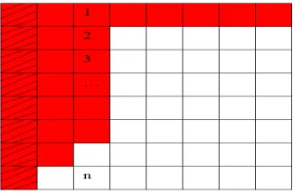
Wavelet transformation entails transformation of image data horizontally first and then vertically. Here the image plane is divided into n horizontal sections which are horizontally transformed concurrently. After then the image is divided into
n vertical sections which are then vertically transformed concurrently. It is not a must that the number of horizontal sections is equal to the number of vertical sections. Figure 1 below illustrates the method.
This lets the possibility for vertical transformation to begin on some vertical sections before horizontal transformation in all sections is completed. Vertical sections that are already horizontally transformed can be vertically transformed as illustrated in Figure 2. That allows the possibility for threads that completed horizontal transformation to go on to vertical transformation without having to wait on other threads to complete horizontal transformation. The red color indicates sections of image data that are horizontally transformed. The white color indicates sections of image data that are not yet horizontally transformed [16]. The red vertical section with line stripes can be assigned to a thread for vertical transformation. Before a vertical section is available for transformation, one condition that must be met is that all horizontal sections transform n size data horizontally such that an n wide vertical section is available with all data points already horizontally transformed.
Image Data
1
2
…
n
[image:3.612.310.570.269.409.2]1 2 … n
[image:3.612.348.510.619.726.2]Figure 1: Image Division
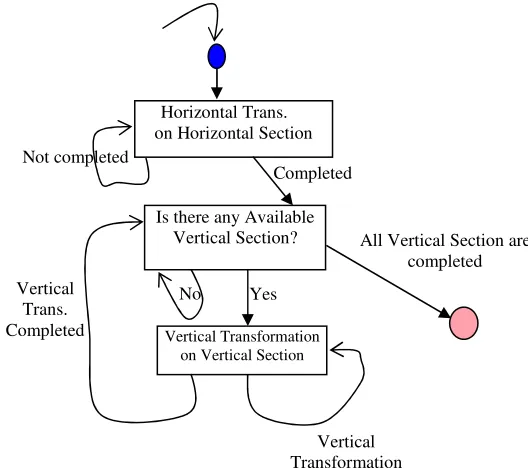
Now let us discuss about the transition system of the model for parallelizing the system. Before that, let us have a brief look at transition system and Kripke Structure that are needed to understand the term “model”. A transition system is a structure TS = (S, S0, R) where, S is a finite set of states; S0 ⊆ S is the set of initial states and R ⊆ S × S is a transition relation which must be total i.e. for every s in S there exists s’ in S such that (s, s’) is in R (∀ s ∈ S ∃ s’ ∈ S . (s, s’) ∈ R). On the other hand, M = (S, S0, R, AP, L) is a Kripke Structure; where (S, S0, R) is a transition system. AP is a finite set of atomic propositions (each proposition corresponds to a variable in the model) and L is a labeling function. It labels each state with a set of atomic propositions that are true in that state. The atomic propositions and L together convert a transitions system into a model. The foremost step to verify a system is to specify the properties that the system should have. For example, we may want to show that some concurrent program never deadlocks. These properties are represented by temporal logic. Computational Tree Logic (CTL) is one of the versions of temporal logic. It is currently one of the popular frameworks used in verifying properties of concurrent system. Once we know which properties are important, the second step is to construct a formal model for that system. The model should capture those properties that must be considered for the establishment of correctness. Model checking includes the traversing the state transition graph (Kripke Structure) and of verifying that if it satisfies the formula representing the property or not, more concisely, the system is a model of the property or not. Each CTL formula is either true or false in a given state of the Kripke Structure. Its truth is evaluated from the truth of its sub-formulae in a recursive fashion, until one reaches atomic propositions that are either true or false in a given state. A formula is satisfied by a system if it is true for all the initial states of the system. Mathematically, say, a Kripke Structure K = (S, S0, R, AP, L) (system model) and a CTL formula Ψ (specification of the property) are given. We have to determine if K |= Ψ holds (K is a model of Ψ) or not. K |= Ψ holds iff K, s0 |= Ψ for every s0 ∈ S0. If the property does not hold, the model checker produces a counter example that is an execution path that can not satisfy that formula [17]. Figure 4 shows the state diagram of the parallel model for verification. It illustrates the tasks of a single thread performing horizontal transformation on a horizontal section and vertical transformation on zero or more vertical sections.
The assertion for the verification is that at any time, the vertical transformation does not start on a vertical section that is not horizontally transformed. In Figure 3, the vertical transformation can start in vertical sections V0 and V1 but not in V2 through V7.
IV. CONCLUSION
Though the DCT-based image compression method performs well at moderate bit rates, the image quality degrades rapidly at higher compression ratios. This is due to the artifacts resulting from the block-based DCT scheme. On the contrary, wavelet-based compression technique provides substantial enhancement in picture quality at low bit rates due to overlapping basis functions and better energy compaction property of wavelet transforms. This paper presents some mathematical background of compression technique mainly based on the wavelet as well as the compression method. Also, a model for parallelizing the method has been proposed. As for the future work, the parallel model may be enhanced and modelled in some formal verification techniques such as SPIN, SMV etc to find out the possible bug in the parallel design.
REFERENCES
[1] http://www.debugmode.com/imagecmp
/
[2] Jayant, N. and Noll, P., Digital Coding of Waveforms: Principles and Applications to Speech and Video, NJ: Prentice-Hall, 1984.
[3] Polikar, R. B. "Wavelet Tutorial Part I, II, III,IV",http://users.rowan.edu/~polikar/WAVELETS/WTt utorial.html, 2003.
[4] David Salomon, Data Compression the Complete Reference, 2nd Ed. Springer, 2002.
[5] Michael B.Martin, Application of Wavelets to image
No Yes
Completed
Horizontal Trans. on Horizontal Section
Not completed
All Vertical Section are completed Vertical
Trans.
Completed Vertical Transformation
on Vertical Section
Is there any Available Vertical Section?
[image:4.612.319.583.118.356.2]Vertical Transformation
Figure 4: State diagram of single thread
[image:4.612.55.263.567.702.2]Compression, M.S. Thesis, Blacksburg Virigina, 1999. [6] Jayant, N., Johnston, J., and Safranek, R., "Signal
compression based on models of human perception" in Proc. IEEE, vol. 81, pp. 1385–1422, October 1993. [7] Rao, K. R. and Yip, P., Discrete Cosine Transform:
Algorithms, Advantages and Applications. San Diego, CA: Academic, 1990.
[8] Gortler. S., Schröder, P., Cohen, M., and Hanrahan, P., "Wavelet Radiosity", in Proc. SIGGRAPH, pp. 221-230, 1993.
[9] Berman, D., Bartell, J. and Salesin, D., "Multiresolution Painting and Compositing", in Proc. SIGGRAPH, pp. 85-90, 1994.
[10]Finkelstein. A. and Salesin, D., "Multiresolution Curves", in Proc. SIGGRAPH, pp.261-268, 1994.
[11]Eck, M., DeRose, T., Duchamp, T., Hoppe, H., Lounsberry, M. and Stuetzle, W., "Multiresolution Analysis of Arbitrary Meshes", in Proc. SIGGRAPH, pp. 173-182, 1995.
[12]Lippert, L. and Gross, M., "Fast Wavelet Based Volume Rendering by Accumulation of Transparent Texture Maps", in Proc. EUROGRAPHICS, pp. 431-443, 1995. [13]Jacobs, C., Finkelstein, A. and Salesin, D., "Fast
Multiresolution Image Querying", in Proc. SIGGRAPH, pp. 277-286, 1995.
[14]Kamrul Hasan Talukder and Koichi Harada,
"Development and Performance Analysis of an Adaptive and Scalable Image Compression Scheme with Wavelets", Published in the Proc. of ICICT, March 2007, BUET, Dhaka, Bangladesh, pp. 250-253, ISBN: 984-32-3394-8. [15]Eric J. Stollnitz, Tony D. Derose and David H. Salesin,
“Wavelets for Computer Graphics”, Morgan Kaufmann Publishers, Inc., San Francisco.
[16]http://www.cis.ksu.edu/~hadassa.