Learning part-of-speech taggers with inter-annotator agreement loss
Barbara Plank, Dirk Hovy, Anders Søgaard Center for Language Technology University of Copenhagen, Denmark Njalsgade 140, DK-2300 Copenhagen S
[email protected],[email protected],[email protected]
Abstract
In natural language processing (NLP) an-notation projects, we use inter-annotator agreement measures and annotation guide-lines to ensure consistent annotations. However, annotation guidelines often make linguistically debatable and even somewhat arbitrary decisions, and inter-annotator agreement is often less than perfect. While annotation projects usu-ally specify how to deal with linguisti-cally debatable phenomena, annotator dis-agreements typically still stem from these “hard” cases. This indicates that some er-rors are more debatable than others. In this paper, we use small samples of doubly-annotated part-of-speech (POS) data for Twitter to estimate annotation reliability and show how those metrics oflikely inter-annotator agreement can be implemented in the loss functions of POS taggers. We find that these cost-sensitive algorithms perform better across annotation projects and, more surprisingly, even on data an-notated according to the same guidelines. Finally, we show that POS tagging mod-els sensitive to inter-annotator agreement perform better on the downstream task of chunking.
1 Introduction
POS-annotated corpora and treebanks are collec-tions of sentences analyzed by linguists accord-ing to some laccord-inguistic theory. The specific choice of linguistic theory has dramatic effects on down-stream performance in NLP tasks that rely on syn-tactic features (Elming et al., 2013). Variation across annotated corpora in linguistic theory also poses challenges to intrinsic evaluation (Schwartz et al., 2011; Tsarfaty et al., 2012), as well as
for languages where available resources are mu-tually inconsistent (Johansson, 2013). Unfortu-nately, there is no grand unifying linguistic the-ory of how to analyze the structure of sentences. While linguists agree on certain things, there is still a wide range of unresolved questions. Con-sider the following sentence:
(1) @GaryMurphyDCU of @DemMattersIRL will take part in a panel discussion on Octo-ber 10th re the aftermath of #seanref . . .
While linguists will agree that inis a preposi-tion, andpanel discussiona compound noun, they are likely to disagree whetherwillis heading the main verbtakeor vice versa. Even at a more basic level of analysis, it is not completely clear how to assign POS tags to each word in this sentence: is part a particle or a noun; is 10tha numeral or a noun?
Some linguistic controversies may be resolved by changing the vocabulary of linguistic theory, e.g., by leaving out numerals or introducing ad hoc parts of speech, e.g. for English to (Marcus et al., 1993) or words ending in -ing (Manning, 2011). However, standardized label sets have practical advantages in NLP (Zeman and Resnik, 2008; Zeman, 2010; Das and Petrov, 2011; Petrov et al., 2012; McDonald et al., 2013).
For these and other reasons, our annotators (even when they are trained linguists) often dis-agree on how to analyze sentences. The strategy in most previous work in NLP has been to monitor and later resolve disagreements, so that the final labels are assumed to be reliable when used as in-put to machine learning models.
Our approach
Instead of glossing over those annotation disagree-ments, we consider what happens if we embrace the uncertainty exhibited by human annotators
when learning predictive models from the anno-tated data.
To achieve this, we incorporate the uncertainty exhibited by annotators in the training of our model. We measure inter-annotator agreement on small samples of data, then incorporate this in the loss function of a structured learner to reflect the confidence we can put in the annotations. This provides us with cost-sensitive online learning al-gorithms for inducing models from annotated data that take inter-annotator agreement into consider-ation.
Specifically, we use online structured percep-tron with drop-out, which has previously been ap-plied to POS tagging and is known to be robust across samples and domains (Søgaard, 2013a). We incorporate the inter-annotator agreement in the loss function either as inter-annotator F1-scores or as the confusion probability between annota-tors (see Section 3 below for a more detailed de-scription). We use a small amounts of doubly-annotated Twitter data to estimateF1-scores and confusion probabilities, and incorporate them dur-ing traindur-ing via a modified loss function. Specif-ically, we use POS annotations made by two an-notators on a set of 500 newly sampled tweets to estimate our agreement scores, and train mod-els on existing Twitter data sets (described be-low). We evaluate the effect of our modified training by measuring intrinsic as well as down-stream performance of the resulting models on two tasks, namely named entity recognition (NER) and chunking, which both use POS tags as input fea-tures.
2 POS-annotated Twitter data sets
The vast majority of POS-annotated resources across languages contain mostly newswire text. Some annotated Twitter data sets do exist for En-glish. Ritter et al. (2011) present a manually an-notated data set of 16 thousand tokens. They do not report inter-annotator agreement. Gimpel et al. (2011) annotated about 26 thousand tokens and report a raw agreement of 92%. Foster et al. (2011) annotated smaller portions of data for cross-domain evaluation purposes. We refer to the data as RITTER, GIMPELand FOSTERbelow.
In our experiments, we use the RITTER splits provided by Derczynski et al. (2013), and the October splits of the GIMPEL data set, version 0.3. We train our models on the concatenation of
RITTER-TRAINand GIMPEL-TRAINand evaluate them on the remaining data, the dev and test set provided by Foster et al. (2011) as well as an in-house annotated data set of 3k tokens (see below). The three annotation efforts (Ritter et al., 2011; Gimpel et al., 2011; Foster et al., 2011) all used different tagsets, however, and they also differ in tokenization, as well as a wide range of linguistic decisions. We mapped all the three corpora to the universal tagset provided by Petrov et al. (2012) and used the same dummy symbols for numbers, URLs, etc., in all the data sets. Following (Fos-ter et al., 2011), we consider URLs, usernames and hashtags asNOUN. We did not change the tok-enization.
The data sets differ in how they analyze many of the linguistically hard cases. Consider, for exam-ple, the analysis ofwill you come out toin GIM -PEL and RITTER (Figure 1, top). While Gimpel et al. (2011) tagoutandto as adpositions, Ritter et al. (2011) consider them particles. What is the right analysis depends on the compositionality of the construction and the linguistic theory one sub-scribes to.
Other differences include the analysis of abbre-viations (PRT in GIMPEL; X in RITTERand FOS -TER), colon (X in GIMPEL; punctuation in RIT -TERand FOSTER), and emoticons, which can take multiple parts of speech in GIMPEL, but are al-ways X in RITTER, while they are absent in FOS -TER. GIMPEL-TRAIN and RITTER-TRAIN are also internally inconsistent. See the bottom of Fig-ure 1 for examples and Hovy et al. (2014) for a more detailed discussion on differences between the data sets.
. . . will you come out to the . . .
GIMPEL VERB PRON VERB ADP ADP DET
RITTER VERB PRON VERB PRT PRT DET
RITTER
. . . you/PRONit/PRON comes/VERB out/ADPcome/VERB out/PRT nov/NOUNto/PRT . . .
GIMPEL
[image:3.595.90.509.63.219.2]. . . Journalists/NOUN and/CONJAdvances/NOUN and/CONJ Social/NOUN Media/NOUNSocial/ADJ Media/NOUN experts/NOUN.../X . . .
Figure 1: Annotation differences between (top) and within (bottom) two available Twitter POS data sets.
or where they had flagged their choice as debat-able. The final data set (lowlands.test), referred below to as INHOUSE, contained 3,064 tokens (200 tweets) and is publicly available
at http://bitbucket.org/lowlands/
costsensitive-data/, along with the data
used to compute inter-annotator agreement scores for learning cost-sensitive taggers, described in the next section.
3 Computing agreement scores
Gimpel et al. (2011) used 72 doubly-annotated tweets to estimate inter-annotator agreement, and we also use doubly-annotated data to compute agreement scores. We randomly sampled 500 tweets for this purpose. Each tweet was anno-tated by two annotators, again using the univer-sal tag set (Petrov et al., 2012). All annotators were encouraged to use their own best judgment rather than following guidelines or discussing dif-ficult cases with each other. This is in contrast to Gimpel et al. (2011), who used annotation guide-lines. The average inter-annotator agreement was 0.88 for raw agreement, and 0.84 for Cohen’s κ. Gimpel et al. (2011) report a raw agreement of 0.92.
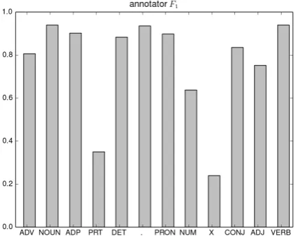
We use two metrics to provide a more detailed picture of inter-annotator agreement, namely F1-scoresbetween annotators on individual parts of speech, andtag confusion probabilities, which we derive from confusion matrices.
The F1-score relates to precision and recall in the usual way, i.e, as the harmonic mean between those two measure. In more detail, given two annotators A1 andA2, we say the precision
Figure 2: Inter-annotator F1-scores estimated from 500 tweets.
ofA1 relative toA2 with respect to POS tagT in
some data setX, denotedPrecT(A1(X), A2(X)),
is the number of tokens bothA1andA2predict to
beT over the number of timesA1predicts a token
to be T. Similarly, we define the recall with re-spect to some tagT, i.e.,RecT(A1(X), A2(X)),
as the number of tokens both A1 andA2 predict
to be T over the number of times A2 predicts
a token to be T. The only difference with respect to standard precision and recall is that the gold standard is replaced by a second anno-tator, A2. Note that PrecT(A1(X), A2(X)) = RecT(A2(X), A1(X)). It follows from all of
the above that the F1-score is symmetrical, i.e., F1T(A1(X), A2(X)) =F1T(A2(X), A1(X)).
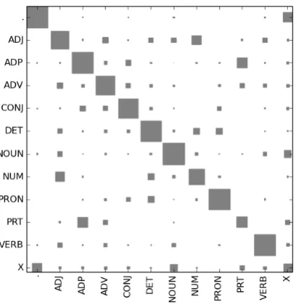
[image:3.595.309.525.264.436.2]agree-Figure 3: Confusion matrix of POS tags obtained from 500 doubly-annotated tweets.
ment is low, for instance, for particles, numerals and the X tag.
We compute tag confusion probabilities from a confusion matrix over POS tags like the one in Figure 3. From such a matrix, we compute the probability of confusing two tags t1 and t2 for some data point x,
i.e. P({A1(x), A2(x)} = {t1, t2}) as the
mean of P(A1(x) = t1, A2(x) = t2) and P(A1(x) = t2, A2(x) = t1), e.g., the confusion
probability of two tags is the mean of the prob-ability that annotatorA1 assigns one tag andA2
another, and vice versa.
We experiment with both agreement scores (F1 and confusion matrix probabilities) to augment the loss function in our learner. The next section de-scribes this modification in detail.
4 Inter-annotator agreement loss
We briefly introduce the cost-sensitive perceptron classifier. Consider the weighted perceptron loss on ourith examplehxi, yii(with learning rateα=
1),Lw(hxi, yii):
γ(sign(w·xi), yi) max(0,−yiw·xi)
In a non-cost-sensitive classifier, the weight function γ(yj, yi) = 1 for 1 ≤ i ≤ N. The
1: X={hxi, yii}Ni=1withxi =hx1i, . . . , xmi i
2: Iiterations 3: w=h0im 4: foriter ∈I do 5: for1≤i≤N do
6: yˆ= arg maxy∈Yw·Φ(xi, y)
7: w←w+γ(ˆy, yi)[Φ(xi, yi)−Φ(xi,yˆ)]
8: w∗+ =w
9: end for
10: end for
[image:4.595.311.524.61.213.2]11: return w∗/= (N ×I)
Figure 4: Cost-sensitive structured perceptron (see Section 3 for weight functionsγ).
two cost-sensitive systems proposed only differ in how we formulateγ(·,·). In one model, the loss is weighted by the inter-annotatorF1of the gold tag in question. This boils down to
γ(yj, yi) =F1yi(A1(X), A2(X))
whereXis the small sample of held-out data used to estimate inter-annotator agreement. Note that in this formulation, the predicted label is not taken into consideration.
The second model is slightly more expressive and takesboththe gold and predicted tags into ac-count. It basically weights the loss by how likely the gold and predicted tag are to be mistaken for each other, i.e., (the inverse of) their confusion probability:
γ(yj, yi)) = 1−P({A1(X), A2(X)}={yj, yi})
In both loss functions, a lower gamma value means that the tags are more likely to be confused by a pair of annotators. In this case, the update is smaller. In contrast, the learner incurs greater loss when easy tags are confused.
It is straight-forward to extend these cost-sensitive loss functions to the structured percep-tron (Collins, 2002). In Figure 4, we provide the pseudocode for the cost-sensitive structured online learning algorithm. We refer to the cost-sensitive structured learners as F1- andCM-weighted be-low.
5 Experiments
[image:4.595.78.290.62.279.2]using a drop-out rate of 0.1 for regularization, fol-lowing Søgaard (2013a). We use the LXMLS toolkit implementation1 with default parameters. We present learning curves across iterations, and only set parameters using held-out data for our downstream experiments.2
5.1 Results
Our results are presented in Figure 5. The top left graph plots accuracy on the training data per iter-ation. We see that CM-weighting does not hurt training data accuracy. The reason may be that the cost-sensitive learner does not try (as hard) to optimize performance on inconsistent annotations. The next two plots (upper mid and upper right) show accuracy over epochs on in-sample evalua-tion data, i.e., GIMPEL-DEV and RITTER-TEST. Again, the CM-weighted learner performs better than our baseline model, while the F1-weighted learner performs much worse.
The interesting results are the evaluations on out-of-sample evaluation data sets (FOSTER and IN-HOUSE) - lower part of Figure 5. Here, both our learners are competitive, but overall it is clear that the CM-weighted learner performs best. It consistently improves over the baseline and F 1-weighting. The former is much more expressive as it takes confusion probabilities into account and does not only update based on gold-label uncer-tainty, as is the case with theF1-weighted learner.
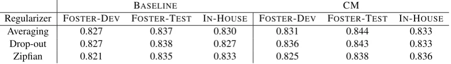
5.2 Robustness across regularizers
Discriminative learning typically benefits from regularization to prevent overfitting. The simplest is the averaged perceptron, but various other meth-ods have been suggested in the literature.
We use structured perceptron with drop-out, but results are relatively robust across other regular-ization methods. Drop-out works by randomly dropping a fraction of the active features in each iteration, thus preventing overfitting. Table 1 shows the results for using different regularizers, in particular, Zipfian corruptions (Søgaard, 2013b) and averaging. While there are minor differences across data sets and regularizers, we observe that the corresponding cell using the loss function sug-gested in this paper (CM) always performs better than the baseline method.
1https://github.com/gracaninja/
lxmls-toolkit/
2In this case, we use FOSTER-DEV as our development
data to avoid in-sample bias.
6 Downstream evaluation
We have seen that our POS tagging model im-proves over the baseline model on three out-of-sample test sets. The question remains whether training a POS tagger that takes inter-annotator agreement scores into consideration is also effec-tive on downstream tasks. Therefore, we eval-uate our best model, the CM-weighted learner, in two downstream tasks: shallow parsing—also known as chunking—and named entity recogni-tion (NER).
For the downstream evaluation, we used the baseline and CM models trained over 13 epochs, as they performed best on FOSTER-DEV(cf. Fig-ure 5). Thus, parameters were optimized only on POS tagging data, not on the downstream evalu-ation tasks. We use a publicly available imple-mentation of conditional random fields (Lafferty et al., 2001)3 for the chunking and NER exper-iments, and provide the POS tags from our CM learner as features.
6.1 Chunking
The set of features for chunking include informa-tion from tokens and POS tags, following Sha and Pereira (2003).
We train the chunker on Twitter data (Ritter et al., 2011), more specifically, the 70/30 train/test split provided by Derczynski et al. (2013) for POS tagging, as the original authors performed cross validation. We train on the 70% Twitter data (11k tokens) and evaluate on the remaining 30%, as well as on the test data from Foster et al. (2011). The FOSTER data was originally annotated for POS and constituency tree information. We con-verted it to chunks using publicly available conver-sion software.4 Part-of-speech tags are the ones assigned by our cost-sensitive (CM) POS model trained on Twitter data, the concatenation of Gim-pel and 70% Ritter training data. We did not in-clude the CoNLL 2000 training data (newswire text), since adding it did not substantially improve chunking performance on tweets, as also shown in (Ritter et al., 2011).
The results for chunking are given in Ta-ble 2. They show that using the POS tagging model (CM) trained to be more sensitive to inter-annotator agreement improves performance over
3http://crfpp.googlecode.com 4http://ilk.uvt.nl/team/sabine/
5 10 15 20 25 Epochs
74 75 76 77 78 79 80 81 82
Accuracy
(%)
TRAINING
BASELINE
F1 CM
5 10 15 20 25
Epochs
77.5 78.0 78.5 79.0 79.5 80.0 80.5
Accuracy
(%)
GIMPEL-DEV
BASELINE
F1 CM
5 10 15 20 25
Epochs
83.5 84.0 84.5 85.0 85.5 86.0 86.5 87.0
Accuracy
(%)
RITTER-TEST
BASELINE
F1 CM
5 10 15 20 25
Epochs
81.0 81.5 82.0 82.5 83.0 83.5 84.0
Accuracy
(%)
FOSTER-DEV
BASELINE
F1 CM
5 10 15 20 25
Epochs
82.5 83.0 83.5 84.0 84.5 85.0
Accuracy
(%)
FOSTER-TEST
BASELINE
F1 CM
5 10 15 20 25
Epochs
82.2 82.4 82.6 82.8 83.0 83.2 83.4 83.6 83.8 84.0
Accuracy
(%)
IN-HOUSE
BASELINE
[image:6.595.76.525.95.453.2]F1 CM
Figure 5: POS accuracy for the three models: baseline, confusion matrix loss (CM) andF1-weighted (F1) loss for increased number of training epochs. Top row: in-sample accuracy on training (left) and in-sample evaluation datasets (center, right). Bottom row: out-of-sample accuracy on various data sets. CM is robust on both in-sample and out-of-sample data.
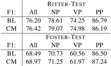
RITTER-TEST
F1: All NP VP PP
BL 76.20 78.61 74.25 86.79 CM 76.42 79.07 74.98 86.19
FOSTER-TEST
F1: All NP VP PP
BL 68.49 70.73 60.56 86.50 CM 68.97 71.25 61.97 87.24 Table 2: Downstream results on chunking. Overall F1 score (All) as well as F1 for NP, VP and PP.
the baseline (BL) for the downstream task of chunking. Overall chunking F1 score improves.
[image:6.595.89.273.565.675.2]BASELINE CM
Regularizer FOSTER-DEV FOSTER-TEST IN-HOUSE FOSTER-DEV FOSTER-TEST IN-HOUSE
Averaging 0.827 0.837 0.830 0.831 0.844 0.833
Drop-out 0.827 0.838 0.827 0.836 0.843 0.833
[image:7.595.73.525.64.128.2]Zipfian 0.821 0.835 0.833 0.825 0.838 0.836
Table 1: Results across regularizers (after 13 epochs).
linguistic theories nor annotators do agree upon.
6.2 NER
In the previous section, we saw positive effects of cost-sensitive POS tagging for chunking, and here we evaluate it on another downstream task, NER.
For the named entity recognition setup, we use commonly used features, in particular features for word tokens, orthographic features like the presence of hyphens, digits, single quotes, up-per/lowercase, 3 character prefix and suffix infor-mation. Moreover, we add Brown word cluster features that use 2,4,6,8,..,16 bitstring prefixes es-timated from a large Twitter corpus (Owoputi et al., 2013).5
For NER, we do not have access to carefully annotated Twitter data for training, but rely on the crowdsourced annotations described in Finin et al. (2010). We use the concatenation of the CoNLL 2003 training split of annotated data from the Reuters corpus and the Finin data for training, as in this case training on the union resulted in a model that is substantially better than training on any of the individual data sets. For evaluation, we have three Twitter data set. We use the recently published data set from the MSM 2013 challenge (29k tokens)6, the data set of Ritter et al. (2011) used also by Fromheide et al. (2014) (46k tokens), as well as an in-house annotated data set (20k to-kens) (Fromheide et al., 2014).
F1: RITTER MSM IN-HOUSE BL 78.20 82.25 82.58 CM 78.30 82.00 82.77
Table 3: Downstream results for named entity recognition (F1 scores).
Table 3 shows the result of using our POS mod-els in downstream NER evaluation. Here we ob-serve mixed results. The cost-sensitive model is
5http://www.ark.cs.cmu.edu/TweetNLP/ 6http://oak.dcs.shef.ac.uk/msm2013/ie_
challenge/
able to improve performance on two out of the three test sets, while being slightly below baseline performance on the MSM challenge data. Note that in contrast to chunking, POS tags are just one of the many features used for NER (albeit an im-portant one), which might be part of the reason why the picture looks slightly different from what we observed above on chunking.
7 Related work
Cost-sensitive learning takes costs, such as mis-classification cost, into consideration. That is, each instance that is not classified correctly during the learning process may contribute differently to the overall error. Geibel and Wysotzki (2003) in-troduce instance-dependent cost values for the per-ceptron algorithm and apply it to a set of binary classification problems. We focus here on struc-tured problems and propose cost-sensitive learn-ing for POS tagglearn-ing uslearn-ing the structured percep-tron algorithm. In a similar spirit, Higashiyama et al. (2013) applied cost-sensitive learning to the structured perceptron for an entity recognition task in the medical domain. They consider the dis-tance between the predicted and true label se-quence smoothed by a parameter that they esti-mate on a development set. This means that the entire sequence is scored at once, while we update on a per-label basis.
is in a different category. Their approach is thus suitable for a fine-grained tagging scheme and re-quires tuning of the cost parameterσ. We tackle the problem from a different angle by letting the learner abstract away from difficult, inconsistent cases as estimated from inter-annotator scores.
Our approach is also related to the literature on regularization, since our cost-sensitive loss functions are aimed at preventing over-fitting to low-confidence annotations. Søgaard (2013b; 2013a) presented two theories of linguistic varia-tion and perceptron learning algorithms that reg-ularize models to minimize loss under expected variation. Our work is related, but models varia-tions in annotation rather than variavaria-tions in input.
There is a large literature related to the issue of learning from annotator bias. Reidsma and op den Akker (2008) show that differences between anno-tators are not random slips of attention but rather different biases annotators might have, i.e. differ-ent mdiffer-ental conceptions. They show that a classi-fier trained on data from one annotator performed much better on in-sample (same annotator) data than on data of any other annotator. They propose two ways to address this problem: i) to identify subsets of the data that show higher inter-annotator agreement and use only that for training (e.g. for speaker address identification they restrict the data to instances where at least one person is in the focus of attention); ii) if available, to train sepa-rate models on data annotated by different anno-tators and combine them through voting. The lat-ter comes at the cost of recall, because they de-liberately chose the classifier to abstain in non-consensus cases.
In a similar vein, Klebanov and Beigman (2009) divide the instance space into easy and hard cases, i.e. easy cases are reliably annotated, whereas items that are hard show confusion and disagree-ment. Hard cases are assumed to be annotated by individual annotator’s coin-flips, and thus can-not be assumed to be uniformly distributed (Kle-banov and Beigman, 2009). They show that learn-ing with annotator noise can have deterioratlearn-ing ef-fect at test time, and thus propose to remove hard cases, both at test time (Klebanov and Beigman, 2009) and training time (Beigman and Klebanov, 2009).
In general, it is important to analyze the data and check for label biases, as a machine learner is greatly affected by annotator noise that is not
ran-dom but systematic (Reidsma and Carletta, 2008). However, rather than training on subsets of data or training separate models – which all implicitly as-sume that there is a large amount of training data available – we propose to integrate inter-annotator biases directly into the loss function.
Regarding measurements for agreements, sev-eral scores have been suggested in the literature. Apart from the simple agreement measure, which records how often annotators choose the same value for an item, there are several statistics that qualify this measure by adjusting for other fac-tors, such as Cohen’sκ(Cohen and others, 1960), theG-index score (Holley and Guilford, 1964), or Krippendorff’sα (Krippendorf, 2004). However, most of these scores are sensitive to the label dis-tribution, missing values, and other circumstances. The measure used in this paper is less affected by these factors, but manages to give us a good un-derstanding of the agreement.
8 Conclusion
In NLP, we use a variety of measures to assess and control annotator disagreement to produce ho-mogenous final annotations. This masks the fact that some annotations are more reliable than oth-ers, and which is thus not reflected in learned pre-dictors. We incorporate the annotator uncertainty on certain labels by measuring annotator agree-ment and use it in the modified loss function of a structured perceptron. We show that this ap-proach works well independent of regularization, both on in-sample and out-of-sample data. More-over, when evaluating the models trained with our loss function on downstream tasks, we observe im-provements on two different tasks. Our results suggest that we need to pay more attention to an-notator confidence when training predictors.
Acknowledgements
We would like to thank the anonymous review-ers and Nathan Schneider for valuable comments and feedback. This research is funded by the ERC Starting Grant LOWLANDS No. 313695.
References
Eyal Beigman and Beata Klebanov. 2009. Learning with annotation noise. InACL.
for nominal scales. Educational and psychological measurement, 20(1):37–46.
Michael Collins. 2002. Discriminative training meth-ods for hidden markov models: Theory and experi-ments with perceptron algorithms. InEMNLP.
Dipanjan Das and Slav Petrov. 2011. Unsupervised part-of-speech tagging with bilingual graph-based projections. InACL.
Leon Derczynski, Alan Ritter, Sam Clark, and Kalina Bontcheva. 2013. Twitter part-of-speech tagging for all: overcoming sparse and noisy data. In RANLP.
Jakob Elming, Anders Johannsen, Sigrid Klerke, Emanuele Lapponi, Hector Martinez, and Anders Søgaard. 2013. Down-stream effects of tree-to-dependency conversions. InNAACL.
Tim Finin, Will Murnane, Anand Karandikar, Nicholas Keller, Justin Martineau, and Mark Dredze. 2010. Annotating named entities in Twitter data with crowdsourcing. InNAACL-HLT 2010 Workshop on Creating Speech and Language Data with Amazon’s Mechanical Turk.
Jennifer Foster, Ozlem Cetinoglu, Joachim Wagner, Josef Le Roux, Joakim Nivre, Deirde Hogan, and Josef van Genabith. 2011. From news to comments: Resources and benchmarks for parsing the language of Web 2.0. InIJCNLP.
Hege Fromheide, Dirk Hovy, and Anders Søgaard. 2014. Crowdsourcing and annotating NER for Twit-ter #drift. InProceedings of LREC 2014.
Peter Geibel and Fritz Wysotzki. 2003. Perceptron based learning with example dependent and noisy costs. InICML.
Kevin Gimpel, Nathan Schneider, Brendan O’Connor, Dipanjan Das, Daniel Mills, Jacob Eisenstein, Michael Heilman, Dani Yogatama, Jeffrey Flanigan, and Noah A. Smith. 2011. Part-of-speech tagging for twitter: Annotation, features, and experiments. InACL.
Shohei Higashiyama, Kazuhiro Seki, and Kuniaki Ue-hara. 2013. Clinical entity recognition using cost-sensitive structured perceptron for NTCIR-10 MedNLP. InNTCIR.
Jasper Wilson Holley and Joy Paul Guilford. 1964. A Note on the G-Index of Agreement. Educational and Psychological Measurement, 24(4):749.
Dirk Hovy, Barbara Plank, and Anders Søgaard. 2014. When POS datasets don’t add up: Combatting sam-ple bias. InProceedings of LREC 2014.
Richard Johansson. 2013. Training parsers on incom-patible treebanks. InNAACL.
Beata Klebanov and Eyal Beigman. 2009. From an-notator agreement to noise models. Computational Linguistics, 35(4):495–503.
Klaus Krippendorf, 2004. Content Analysis: An In-troduction to Its Methodology, second edition, chap-ter 11. Sage, Thousand Oaks, CA.
John Lafferty, Andrew McCallum, and Fernando Pereira. 2001. Conditional random fields: prob-abilistic models for segmenting and labeling se-quence data. InICML.
Christopher D Manning. 2011. Part-of-speech tag-ging from 97% to 100%: is it time for some linguis-tics? In Computational Linguistics and Intelligent Text Processing, pages 171–189. Springer.
Mitchell Marcus, Mary Marcinkiewicz, and Beatrice Santorini. 1993. Building a large annotated cor-pus of English: the Penn Treebank. Computational Linguistics, 19(2):313–330.
Ryan McDonald, Joakim Nivre, Yvonne Quirmbach-Brundage, Yoav Goldberg, Dipanjan Das, Kuz-man Ganchev, Keith Hall, Slav Petrov, Hao Zhang, Oscar T¨ackstr¨om, Claudia Bedini, N´uria Bertomeu Castell´o, and Jungmee Lee. 2013. Uni-versal dependency annotation for multilingual pars-ing. InACL.
Olutobi Owoputi, Brendan O’Connor, Chris Dyer, Kevin Gimpel, Nathan Schneider, and Noah A Smith. 2013. Improved part-of-speech tagging for online conversational text with word clusters. In NAACL.
Slav Petrov, Dipanjan Das, and Ryan McDonald. 2012. A universal part-of-speech tagset. InLREC. Dennis Reidsma and Jean Carletta. 2008.
Reliabil-ity measurement without limits. Computational Lin-guistics, 34(3):319–326.
Dennis Reidsma and Rieks op den Akker. 2008. Ex-ploiting ‘subjective’ annotations. In Workshop on Human Judgements in Computational Linguistics, COLING.
Alan Ritter, Sam Clark, Oren Etzioni, et al. 2011. Named entity recognition in tweets: an experimental study. InEMNLP.
Roy Schwartz, Omri Abend, Roi Reichart, and Ari Rappoport. 2011. Neutralizing linguistically prob-lematic annotations in unsupervised dependency parsing evaluation. InACL.
Fei Sha and Fernando Pereira. 2003. Shallow parsing with conditional random fields. InNAACL.
Anders Søgaard. 2013a. Part-of-speech tagging with antagonistic adversaries. InACL.
Hyun-Je Song, Jeong-Woo Son, Tae-Gil Noh, Seong-Bae Park, and Sang-Jo Lee. 2012. A cost sensitive part-of-speech tagging: differentiating serious errors from minor errors. InACL.
Reut Tsarfaty, Joakim Nivre, and Evelina Andersson. 2012. Cross-framework evaluation for statistical parsing. InEACL.
Daniel Zeman and Philip Resnik. 2008. Cross-language parser adaptation between related lan-guages. InIJCNLP.