Proceedings of the 2019 Conference on Empirical Methods in Natural Language Processing
1488
Grounding learning of modifier dynamics:
An application to color naming
Xudong Han♠ Philip Schulz♥
♠University of Melbourne ♥Amazon Research
[email protected] [email protected]
Trevor Cohn♠
Abstract
Grounding is crucial for natural language derstanding. An important subtask is to un-derstand modified color expressions, such as
“dirty blue”. We present a model of color modifiers that, compared with previous addi-tive models in RGB space, learns more com-plex transformations. In addition, we present a model that operates in the HSV color space. We show that certain adjectives are better modeled in that space. To account for all mod-ifiers, we train a hard ensemble model that se-lects a color space depending on the modifier-color pair. Experimental results show signif-icant and consistent improvements compared to the state-of-the-art baseline model.1
1 Introduction
Grounded color descriptions are employed to de-scribe colors which are not covered by basic color terms (Monroe et al.,2017). For instance, “green-ish blue” cannot be expressed by only “blue”
or “green”. Grounded learning of modifiers, as a result, is essential for grounded language understanding problems such as image caption-ing (Karpathy and Fei-Fei,2015), visual question answering (Goyal et al.,2017) and object recogni-tion (van de Sande et al.,2010).
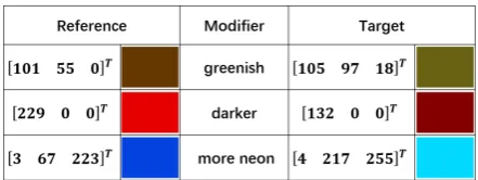
In this paper, we present models that are able to predict the RGB code of a target color given a reference color and a modifier. For exam-ple, as shown in Figure 1, given a reference color code ~r =
101 55 0>
and a modifier
m = “greenish”, our models are trained to pre-dict the target color code~t =
105 97 18> . The state-of-the-art approach for this task (Winn and Muresan, 2018) represents both colors and modifiers as vectors in RGB space, and learns a
[image:1.595.306.527.220.303.2]1Code available at https://github.com/ HanXudong/GLoM
Figure 1: Examples of the grounded modifier mod-elling task, shown in RGB space. Given the reference and modifier, the system must predict the target color.
vector representation of modifiers m~ as part of a simple additive model, ~r +m~ ≈ ~r, in RGB color space. For instance, given the reference color ~r = 229 0 0>, the target color ~t =
132 0 0>
, the modifier m = “darker” is learned as a vector m~ = −97 0 0>
. This model works well when the modifier is well repre-sented as a single vector independent of the ref-erence color,2 but fails to model modifiers with more complex transformations, for example, color related modifiers, like“greenish”, which are bet-ter modelled through color inbet-terpolation.
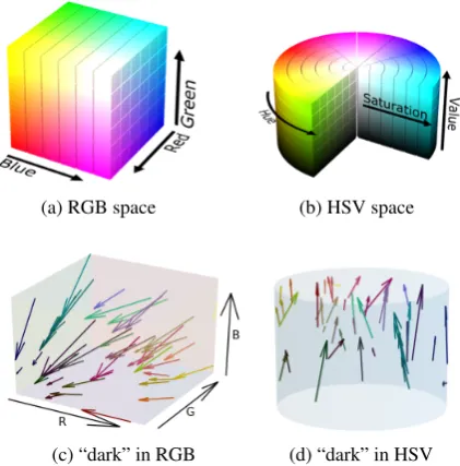
To fit a better model, we assume that there are approximate intersection points for the extension lines of modifier vectors, for instance, Figure 2c shows the“darker”related vectors in RGB space and we can see that the intersection point is ap-proximately
0 0 0>
. On the basis of this, we introduce an RGB model which can learn a transformation matrix and an interpolation point for each modifier.
There are many other color spaces besides RGB, e.g., HSL and HSV (Joblove and Greenberg, 1978;Hanbury,2008), and mapping between such
2Winn and Muresan(2018) parameterizem~ as a function
spaces can be done via invertible transforma-tions (Agoston, 2005). As shown in Figure 2d, for some modifiers, color vectors can be approx-imately parallel in HSV space, thus simplifying the modeling problem. We propose a HSV model using a von-Mises loss, and show that this model outperforms the RGB method for many modifiers. We also present an ensemble model for color space selection, which determines for each modifier the best color space model. Overall our methods sub-stantially outperform prior work, achieving state-of-the-art performance in the grounded color mod-elling task.
2 Methods
Here we describe the methods employed for color modeling. Formally, the task is to predict a target color vector~tin RGB space from a reference color vector~rand a modifier stringm.
2.1 Modeling in RGB space
Baseline Model Winn and Muresan (2018) present a model (WM18) which represents a vec-torm~ ∈R3as a function of (m, ~r) pointing from a reference color vector~rto the target color vector
~t, such that~t= ~r+m~. In the simplest case the modifier m is irrelevant to the reference color~r. This assumption, however, does not hold in all sit-uations. For example, when predicting an instance with the reference vector~r =
193 169 106> and the modifier“greenish”, the outcomeˆtis ex-pected to be177 183 102>, however, WM18 predictsˆt=
195 156 95>
. The cosine simi-larity between(ˆt−~r)and(~t−~r)is−0.76, i.e.,m~
points in the opposite direction to where it should.
RGB Model As shown in Figure 2c, pairs of vectors for the same modifier are often not paral-lel. In theory, such vectors can even be orthogonal: compare “darker red” vs “darker blue”, which fall on different faces of the RGB cube. To model this, we propose a model in RGB space as follows:
~t=M~r+β~ (1)
WhereM ∈R3×3 is a transformation matrix and ~
βis a modifier vector which is designed to capture the information of m. Given an error term ε ∼ N(~0, σI3), the RGB model is trained to minimize the following loss for the log Gaussian likelihood:
(a) RGB space (b) HSV space
[image:2.595.312.523.64.278.2](c) “dark” in RGB (d) “dark” in HSV
Figure 2: 2a: RGB color space. 2b: HSV color space. Ar-rows in2cand2dshow vectors staring from reference colors to target colors in RGB and HSV color spaces. Images2aand
2bby Michael Horvath, available under Creative Commons Attribution-Share Alike 3.0 Unported license.
L= 1
n n
X
i=1
(~ti−tˆi)>(~ti−tˆi) (2)
where~tiis the target vector in each instance andtiˆ
is the prediction.3
Specific Settings Our model generalizes WM18, which can be realized by settingM =I3 andβ~=m~.
Another interesting instance of the model is ob-tained by setting M = (1 − αm)I3 and β~ = αmm~, which we call the Diagonal Covariance (DC) model. In contrast to the RGB model and WM18, which model m~ as a function of ~r and
m, m~ in the DC model does not depend on ~r. Given ~r and m, to predict the~t, our DC model predictsm~ first and then applies a linear transfor-mation to get the target color vector as follows:
~t=~r+αm×(m~ −~r), whereαm ∈[0,1]is a scalar which only depends onm and measures the dis-tance from~rtom~. In the DC modelm~ is the inter-polation point for modifiers, such as 0 0 0>
for the modifier“darker”.
2.2 Modeling in HSV space
Compared with the RGB color space, when mod-eling modifiers in HSV, there are two main
differ-3Although other distributions, such as Beta distribution,
ences: hue is represented as an angular dimension, and the modifier vectors are more frequently par-allel (see Fig2d). As shown in Figure2b, HSV space forms a cylindrical geometry withhueas its angular dimension, with the value red occurring at both 0and 2π. For this reason, modelling the hue with a Gaussian regression loss is not appro-priate. To account for the angularity, we model
“hue”with a von-Mises distribution, with the fol-lowingpdf:
f(h) =
expkcos (h−ˆh)
2πI0(k)
. (3)
The mean valuehˆrepresents the center ofhue di-mension, k indicates the concentration about the mean, andI0(k) is the modified Bessel function of order 0.
When training the model, the parameterkis as-sumed constant, and thus the loss function is:
L= 1− 1 n
n
X
i=1
cos (hi−ˆhi), (4)
wherehiis thehuevalue of the target color in each instance andhiˆ is the prediction.
The second difference to modeling in RGB space is that the modifier behavior is simpler in HSV. For modifiers, vectors from reference col-ors to target colcol-ors are more likely to be parallel (see Figure 2d). As a result, we present an addi-tive model in HSV space where a modifiermwill be modeled as a vector from~rto~t:
~t=~r+m~ (5)
Here m~ is a function of bothm and~r. In addi-tion, modifier modeling will be split into two parts: modeling “hue” dimension as von-Mises distri-bution and other dimensions together as a bivari-ate normal distribution (See Equation 2). Notice that Equation (5) is the same equation as used by WM18, however, here it is applied in a color space that better fits its assumptions.
WM18 is presented and evaluated only in RGB color space. To compare its performance with our models, we transform output into RGB space.
2.3 Ensemble model
An ensemble model is trained to make the final prediction, which we frame as a hard binary choice to select the color space appropriate for the given
modifier. This works by applying the general RGB model and HSV model (Equations 1 and 5) to get their predictions, and converting the HSV pre-dictions into RGB space. Then the hard ensem-ble is trained to predict which color space should be used based on the modifier m and the refer-ence vector~r, using as the learning signal which model prediction had the smallest error against the reference colour for each instance (measured using Delta-E distance, see §3.2). The probabil-ity of the RGB model being selected is: p =
σ(f(m, ~r)), whereσis the logistic sigmoid func-tion andf(m, ~r)is a function of modifiermand reference color~r.
3 Experiments
3.1 Dataset
The dataset4 used to train and evaluate our model includes 415 triples (reference color label,r, mod-ifier, m, and target color label, t) in RGB space presented byWinn and Muresan(2018). Munroe (2010) collected the original dataset consisting of color description pairs collected in an open on-line survey; the dataset was subsequently filtered byMcMahan and Stone(2015). Winn and Mure-san processed color labels and converted pairs to triples with 79 unique reference color labels and 81 unique modifiers.
We train models in both RGB and HSV color space, but samples in WM18 are only presented in RGB space. Because modifiers encode the gen-eral relationship betweenrandtwe use the same approach presented byWinn and Muresan(2018): using the mean value of a set of points to repre-sent a color. A drawback of this approach is that it does not account for our uncertainty about the appropriate RGB encoding for a given color word.
3.2 Experiment Setup
Model configuration: The model presented by Winn and Muresan (2018) is initialized with Google’s pretrained 300-d word2vec embeddings (Mikolov et al., 2013b,a) which are not updated during training. To perform comparable experi-ments, all models in paper are designed with the same trained embedding model. Other pre-trained word embeddings, such as GloVe (Pen-nington et al., 2014) and BERT (Devlin et al., 2019), were also tested but there was no significant
4https://bitbucket.org/o_winn/
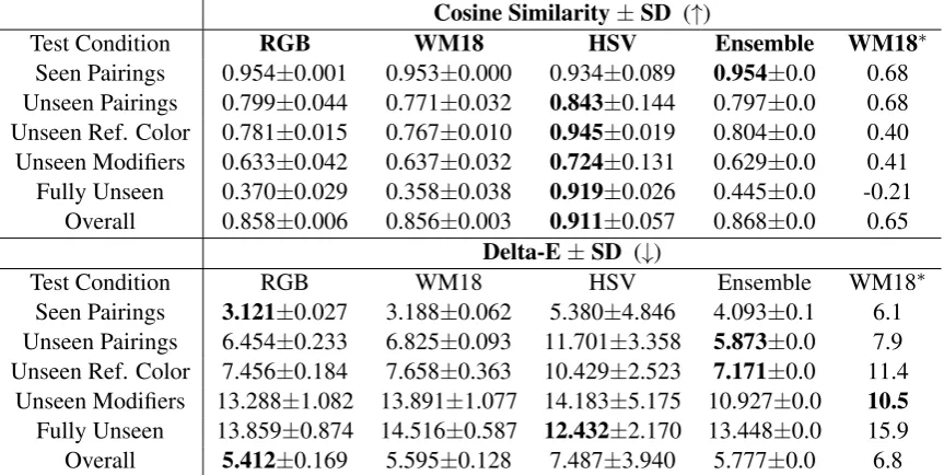
Cosine Similarity±SD (↑)
Test Condition RGB WM18 HSV Ensemble WM18∗
Seen Pairings 0.954±0.001 0.953±0.000 0.934±0.089 0.954±0.0 0.68 Unseen Pairings 0.799±0.044 0.771±0.032 0.843±0.144 0.797±0.0 0.68 Unseen Ref. Color 0.781±0.015 0.767±0.010 0.945±0.019 0.804±0.0 0.40 Unseen Modifiers 0.633±0.042 0.637±0.032 0.724±0.131 0.629±0.0 0.41 Fully Unseen 0.370±0.029 0.358±0.038 0.919±0.026 0.445±0.0 -0.21 Overall 0.858±0.006 0.856±0.003 0.911±0.057 0.868±0.0 0.65
Delta-E±SD (↓)
Test Condition RGB WM18 HSV Ensemble WM18∗
Seen Pairings 3.121±0.027 3.188±0.062 5.380±4.846 4.093±0.1 6.1 Unseen Pairings 6.454±0.233 6.825±0.093 11.701±3.358 5.873±0.0 7.9 Unseen Ref. Color 7.456±0.184 7.658±0.363 10.429±2.523 7.171±0.0 11.4
[image:4.595.84.516.63.280.2]Unseen Modifiers 13.288±1.082 13.891±1.077 14.183±5.175 10.927±0.0 10.5 Fully Unseen 13.859±0.874 14.516±0.587 12.432±2.170 13.448±0.0 15.9 Overall 5.412±0.169 5.595±0.128 7.487±3.940 5.777±0.0 6.8
Table 1: Average cosine similarity score and Delta-E distance over 5 runs. A smaller Delta-E distance means a less significant difference between two colors.Bold: best performance. Hard: the hard ensemble model. WM18∗: the performance from WM18 paper. SeeSupplementary Materialfor example outputs and ensemble analysis.
difference in performance compared to word2vec. Single models are trained over 2000 epochs with batch size 32 and 0.1 learning rate. The hyper-parameters for the ensemble model are as follows: 600 epochs, 32 batch size, and 0.1 learning rate.
Architecture: An input modifier is represented as a vector by word2vec pretrained embeddings and followed by two fully connected layers(F C1 and F C2) with size 32 and 16 respectively. Let h1 be the hidden state of F C2 then h1 = F C2(F C1(~r, Em, ~r) where E are fixed, pre-trained word2vec embeddings. ~r is used as an in-put for both F C1 and F C2. After F C2, all the other layers are based on hidden stateh1.
Evaluation: Following Winn and Muresan (2018), we evaluate the performance in 5 distinct input conditions: (1) Seen Pairings: The triple
(r, m, t) has been seen when training models. (2) Unseen Pairings: Both r and m have been seen in training data, but not the triple (r, m, t). (3) Unseen Ref. Color: r has not been seen in training, while m has been seen. (4) Unseen modifiers: mhas not been seen in training, while
r has been seen. (5)Fully Unseen: Neitherr nor
mhave been seen in training.
Because of the small size of the dataset, we re-port the average performance over 5 runs with dif-ferent random seeds. Two scores, cosine similar-ity, and Delta-E are applied for evaluating the
per-formance. Cosine similarity measures the differ-ence in terms of vector direction in color space and Delta-E is a non-uniformity metric for measuring color differences. Delta-E was first presented as the Euclidean Distance in CIELAB color space (McLaren, 1976). Lower Delta-E values are thus preferable as they indicate better matching of the target color. Luo et al. (2001) present the latest and most accurate CIE color difference metrics, Delta-E 2000, which improve the original formula by taking into account weighting factors and fixing the lightness inaccuracies. Our models are evalu-ated with Delta-E 2000.
3.3 Results
Table1shows the results. Compared with WM18, our RGB model outperforms under all conditions. As we have stated, our model is a generalization of their approach. The more complex transforma-tion matrix in our RGB model is able to learn more information, such as the effects of covariance be-tween color channels, and thus achieves a better performance than WM18. Note that our reimple-mentation of the original WM18 system lead to significantly better performance.5
According to the cosine similarity, the HSV model is superior for most test conditions
(con-5We train the model for many more epochs, which is
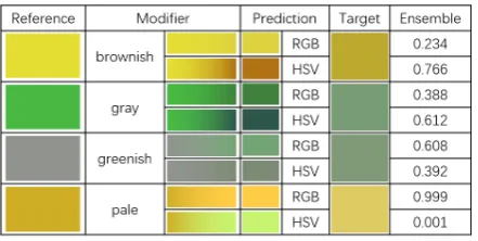
Figure 3: Examples of predictions from RGB, HSV and Ensemble model. The Ensemble column reports the predicted probability of the RGB and HSV models being selected.
firming our hypothesis about simpler modifier be-haviour in this space). However for Delta-E, the RGB model and ensemble perform better. Un-like cosine, Delta-E is sensitive to differences in vector length, and we would argue it is the most appropriate metric because lengths are critical to measuring the extent of lightness and darkness of colors. Accordingly the HSV model does worse under this metric, as it more directly models the direction of color modifiers, but as a consequence this leads to errors in its length predictions. Over-all the ensemble does well according to both met-rics, and has the best performance for several test conditions with Delta-E.
Error Analysis We first focused error analysis on prediction of “Unseen Modifiers” and “Fully Unseen” instances. As shown in Table 1, our models are able to predict target colors given seen modifiers but fail to make predictions for instances with unseen modifiers. All modifiers are rep-resented by word2vec embeddings, and we ex-pect that predictions of unseen modifiers should be close to instances with similar seen modifiers. For example, the prediction of a reference color
~r and modifier“greeny” should be similar to the prediction of the same reference color~rand a sim-ilar seen modifier, e.g. “green”and“greenish”. However, the prediction of“greeny”is more sim-ilar to“bluey”, a consequence of these terms hav-ing highly similar word embeddhav-ings (as do other colour modifiers with a -y suffix, irrespective of their colour). This is related to the problem re-ported inMrkˇsi´c et al.(2016), whereby words and their antonyms often have similar embeddings, as a result of sharing similar distributional contexts. Accordingly for the unseen modifier condition, our model is often misled by attempting to
gener-alise from nearest neighbour modifiers which have a different meaning.
4 Related Work
Baroni and Zamparelli (2010) was the first work to propose an approach to adjective-noun compo-sition (AN) for corpus-based distributional seman-tics which represents nouns as vectors and adjec-tives as matrices nominal vectors. However it is hard to gain an intuition for what the transforma-tion does since these embeddings generally live on a highly structured but unknown manifold. In our case, we operate on colors and we actually know the geometry of the colour spaces we use. This makes it easier for us to interpret the learned map-ping (see Figure2cand2dthat show convergence to a point in RGB and parallelism in HSV space).
5 Conclusion and Future Work
In this paper, we proposed novel models of pre-dicting color based on textual modifiers, incorpo-rating a matrix transformation than the previous largely linear additive method. As well as our more general approach, we exploit the properties of another color space, namely HSV, in which the modifier behaviours are often simpler. Overall our method leads to state of the art performance on a standard dataset.
In future work, we intend to develop more ac-curate modifier representations to allow for better generalisation to unseen modifiers. This might be achieved by using a composition sub-word repre-sentation for modifiers, such as character-level en-coding. Finally, we also strive to acquire larger datasets. This is a crucial step towards comparing the generalization performance of different color-modifier models. Models trained on larger data sets are likely to be more applicable to real-world problems since they learn representations for more color terms.
References
M.K. Agoston. 2005. Computer Graphics and Geo-metric Modelling, pages 300–306. Springer.
Marco Baroni and Roberto Zamparelli. 2010. Nouns are vectors, adjectives are matrices: Representing adjective-noun constructions in semantic space. In
Jacob Devlin, Ming-Wei Chang, Kenton Lee, and Kristina Toutanova. 2019. Bert: Pre-training of deep bidirectional transformers for language under-standing. InProceedings of the 2019 Conference of the North American Chapter of the Association for Computational Linguistics: Human Language Tech-nologies, Volume 1 (Long and Short Papers), pages 4171–4186.
Yash Goyal, Tejas Khot, Douglas Summers-Stay, Dhruv Batra, and Devi Parikh. 2017. Making the V in VQA matter: Elevating the role of image un-derstanding in Visual Question Answering. In Con-ference on Computer Vision and Pattern Recognition (CVPR).
Allan Hanbury. 2008. Constructing cylindrical coor-dinate colour spaces. Pattern Recognition Letters, 29(4):494 – 500.
George H. Joblove and Donald Greenberg. 1978.Color spaces for computer graphics.SIGGRAPH Comput. Graph., 12(3):20–25.
Andrej Karpathy and Li Fei-Fei. 2015. Deep visual-semantic alignments for generating image descrip-tions. InThe IEEE Conference on Computer Vision and Pattern Recognition (CVPR).
M Ronnier Luo, Guihua Cui, and Bryan Rigg. 2001. The development of the cie 2000 colour-difference formula: Ciede2000. Color Research & Appli-cation: Endorsed by Inter-Society Color Council, The Colour Group (Great Britain), Canadian Soci-ety for Color, Color Science Association of Japan, Dutch Society for the Study of Color, The Swedish Colour Centre Foundation, Colour Society of Aus-tralia, Centre Franc¸ais de la Couleur, 26(5):340– 350.
K McLaren. 1976. Xiiithe development of the cie 1976 (l* a* b*) uniform colour space and colour-difference formula. Journal of the Society of Dyers and Colourists, 92(9):338–341.
Brian McMahan and Matthew Stone. 2015. A Bayesian model of grounded color semantics.
Transactions of the Association for Computational Linguistics, 3:103–115.
Tomas Mikolov, Kai Chen, Greg Corrado, and Jeffrey Dean. 2013a. Efficient estimation of word represen-tations in vector space. In 1st International Con-ference on Learning Representations, ICLR 2013, Scottsdale, Arizona, USA, May 2-4, 2013, Workshop Track Proceedings.
Tomas Mikolov, Ilya Sutskever, Kai Chen, Greg S Cor-rado, and Jeff Dean. 2013b. Distributed represen-tations of words and phrases and their composition-ality. In C. J. C. Burges, L. Bottou, M. Welling, Z. Ghahramani, and K. Q. Weinberger, editors, Ad-vances in Neural Information Processing Systems 26, pages 3111–3119. Curran Associates, Inc.
Will Monroe, Robert XD Hawkins, Noah D Goodman, and Christopher Potts. 2017. Colors in context: A pragmatic neural model for grounded language un-derstanding. Transactions of the Association for Computational Linguistics, 5:325–338.
Nikola Mrkˇsi´c, Diarmuid O S´eaghdha, Blaise Thom-son, Milica Gaˇsi´c, Lina Rojas-Barahona, Pei-Hao Su, David Vandyke, Tsung-Hsien Wen, and Steve Young. 2016. Counter-fitting word vec-tors to linguistic constraints. arXiv preprint arXiv:1603.00892.
Randall Munroe. 2010.Color survey results.
Jeffrey Pennington, Richard Socher, and Christo-pher D. Manning. 2014. Glove: Global vectors for word representation. InEmpirical Methods in Nat-ural Language Processing (EMNLP), pages 1532– 1543.
K. van de Sande, T. Gevers, and C. Snoek. 2010. Eval-uating color descriptors for object and scene recog-nition. IEEE Transactions on Pattern Analysis and Machine Intelligence, 32(9):1582–1596.