Proceedings of the 2019 Conference on Empirical Methods in Natural Language Processing and the 9th International Joint Conference on Natural Language Processing, pages 5226–5235,
5226
Document Hashing with Mixture-Prior Generative Models
Wei Dong1, Qinliang Su1, 2∗, Dinghan Shen3, Changyou Chen4
1School of Data and Computer Science, Sun Yat-sen University
2 Guangdong Key Laboratory of Big Data Analysis and Processing, Guangzhou, China 3ECE Department, Duke University 4CSE Department, SUNY at Buffalo
[email protected], [email protected] [email protected], [email protected]
Abstract
Hashing is promising for large-scale informa-tion retrieval tasks thanks to the efficiency of distance evaluation between binary codes. Generative hashing is often used to generate hashing codes in an unsupervised way. How-ever, existing generative hashing methods on-ly considered the use of simple priors, like Gaussian and Bernoulli priors, which limit-s thelimit-se methodlimit-s to further improve their per-formance. In this paper, two mixture-prior generative models are proposed, under the ob-jective to produce high-quality hashing codes for documents. Specifically, a Gaussian mix-ture prior is first imposed onto the variation-al auto-encoder (VAE), followed by a separate step to cast the continuous latent representa-tion of VAE into binary code. To avoid the performance loss caused by the separate cast-ing, a model using a Bernoulli mixture pri-or is further developed, in which an end-to-end training is admitted by resorting to the straight-through (ST) discrete gradient estima-tor. Experimental results on several bench-mark datasets demonstrate that the proposed methods, especially the one using Bernoulli mixture priors, consistently outperform exist-ing ones by a substantial margin.
1 Introduction
Similarity search aims to find items that look most similar to the query one from a huge amount of data (Wang et al.,2018), and are found in exten-sive applications like plagiarism analysis (Stein et al.,2007), collaborative filtering (Koren,2008;
Wang et al.,2016), content-based multimedia re-trieval (Lew et al., 2006), web services (Dong et al.,2004) etc. Semantic hashing is an effective way to accelerate the searching process by rep-resenting every document with a compact binary code. In this way, one only needs to evaluate the
∗
Corresponding author.
hamming distance between binary codes, which is much cheaper than the Euclidean distance calcu-lation in the original feature space.
Existing hashing methods can be roughly divid-ed into data-independent and data-dependent cat-egories. Data-independent methods employ ran-dom projections to construct hash functions with-out any consideration on data characteristics, like the locality sensitive hashing (LSH) algorithm (Datar et al.,2004). On the contrary, data depen-dent hashing seeks to learn a hash function from the given training data in a supervised or an un-supervised way. In the un-supervised case, a deter-ministic function which maps the data to a bina-ry representation is trained by using the provided supervised information (e.g. labels) (Liu et al.,
2012;Shen et al.,2015;Liu et al., 2016). How-ever, the supervised information is often very d-ifficult to obtain or is not available at all. Unsu-pervised hashing seeks to obtain binary represen-tations by leveraging the inherent structure infor-mation in data, such as the spectral hashing (Weiss et al.,2009), graph hashing (Liu et al.,2011), iter-ative quantization (Gong et al.,2013), self-taught hashing (Zhang et al.,2010) etc.
Generative models are often considered as the most natural way for unsupervised representation learning (Miao et al.,2016;Bowman et al.,2015;
2013). To address the issue, the neural architecture for generative semantic hashing (NASH) in (Shen et al.,2018) proposed to use a Bernoulli prior to re-place the Gaussian prior in VDSH, and further use the straight-through (ST) method (Bengio et al.,
2013) to estimate the gradients of functions in-volving binary variables. It is shown that the end-to-end training brings a remarkable performance improvement over the two-stage training method in VDSH. Despite of superior performances, only the simplest priors are used in these models, i.e. Gaussian in VDSH and Bernoulli in NASH. How-ever, it is widely known that priors play an impor-tant role on the performance of generative models (Goyal et al.,2017;Chen et al.,2016;Jiang et al.,
2016).
Motivated by this observation, in this paper, we propose to produce high-quality hashing codes by imposing appropriate mixture priors on generative models. Specifically, we first propose to mod-el documents by a VAE with a Gaussian mixture prior. However, similar to the VDSH, the pro-posed method also requires a separate stage to cast the continuous representation into binary for-m, making it suffer from the same pains of two-stage training. Then we further propose to use a Bernoulli mixture as the prior, in hopes to yield binary representations directly. An end-to-end method is further developed to train the model, by resorting to the straight-through gradient estima-tor for neural networks involving binary random variables. Extensive experiments are conducted on benchmark datasets, which show substantial gains of the proposed mixture-prior methods over exist-ing ones, especially the method with a Bernoulli mixture prior.
2 Semantic Hashing by Imposing Mixture Priors
In this section, we investigate how to obtain similarity-preserved hashing codes by imposing d-ifferent mixture priors on variational encoder.
2.1 Preliminaries on Generative Semantic Hashing
Letx ∈ Z+|V|denote the bag-of-words represen-tation of a document and xi ∈ {0,1}|V| denote
the one-hot vector representation of thei-th word of the document, where |V| denotes the vocabu-lary size. VDSH in (Chaidaroon and Fang,2017) proposed to model a document D, which is
de-fined by a sequence of one-hot word representa-tions{xi}|D|i=1, with the joint PDF
p(D, z) =pθ(D|z)p(z), (1)
where the priorp(z)is the standard Gaussian dis-tributionN(0, I); the likelihood has the factorized formpθ(D|z) =Q
|D|
i=1pθ(xi|z), and
pθ(xi|z) =
exp(zTExi+bi)
P|V|
j=1exp(zTExj+bj)
; (2)
E∈Rm×|V|is a parameter matrix which
connect-s latent repreconnect-sentationzto one-hot representation
xiof thei-th word, withmbeing the dimension of z;biis the bias term andθ={E, b1, ..., b|V|}. It is
known that generative models with better model-ing capability often imply that the obtained latent representations are also more informative.
To increase the modeling ability of (1), we may resort to more complex likelihoodpθ(D|z), such
as using deep neural networks to relate the laten-t z to the observation xi, instead of the simple
softmax function in (2). However, as indicated in (Shen et al.,2018), employing expressive non-linear decoders likely destroy the distance-keeping property, which is essential to yield good hashing codes. In this paper, instead of employing a more complex decoderpθ(D|z), more expressive priors
are leveraged to address this issue.
2.2 Semantic Hashing by Imposing Gaussian Mixture Priors
To begin with, we first replace the standard Gaus-sian priorp(z) =N(0, I)in (1) by the following Gaussian mixture prior
p(z) = K X
k=1
πk· N µk,diag σk2
, (3)
where K is the number of mixture components;
πk is the probability of choosing the k-th
(a) GMSH
ˆ
x ( )
g xf Gaussian
mixture
p
( )
g xf g zq( )
...
1 m s1
x
(b) BMSH
( ( ))g xf
s Bernoulli
mixture mc
z
x
ˆ
...
p
2 ~ ( , ( c)) z¢ z diags
2 logsc
1
m
( )
g zq ¢ ( )
g xf
0.2
0.9
0.4
0.7
0.3
0.1 0
1
0
1
0
0
x
2
m s2
K m sK
2
m
K
m
2
~ ( ,c ( c))
[image:3.595.87.507.66.238.2]z m diags
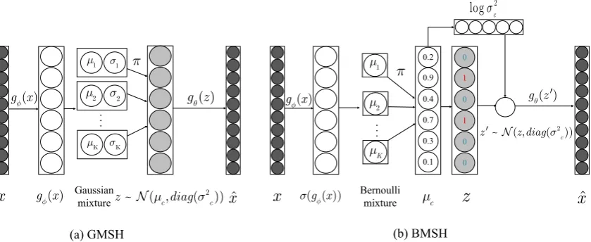
Figure 1: The architectures of the GMSH and BMSH. The data generative process of GMSH is done as follows: (1) Pick a componentc ∈ {1,2, ..., K} fromCat(π)withπ = [π1, π2, ..., πK]; (2) Draw a samplezfrom the
picked Gaussian distributionN µc, diag(σc2)
; (3) Usegθ(z)to decode the samplezinto an observablexˆ. The process of generating data in BMSH can be described as follows: (1) Choose a componentc fromCat(π); (2) Sample a latent vector from the chosen distributionBernoulli(γc); (3) Inject data-dependent noise intoz, and
drawz0fromN(z, diag(σ2
c)); (4) Then use decodergθ(z0)to reconstructxˆ.
distribution N µc,diag σc2
. Thus, the docu-mentDis modelled as
p(D, z, c) =pθ(D|z)p(z|c)p(c), (4)
where p(z|c) = N µc,diag σc2
, p(c) =
Cat(π)andpθ(D|z)is defined the same as (2).
To train the model, we seek to optimize the low-er bound of the log-likelihood
L=Eqφ(z,c|x)
logpθ(D|z)p(z|c)p(c) qφ(z, c|x)
, (5)
whereqφ(z, c|x)is the approximate posterior
dis-tribution of p(z, c|x) parameterized by φ; here
x could be any representation of the documents, like the bag-of-words, TFIDF etc. For the sake of tractability, qφ(z, c|x) is further assumed to
maintain a factorized form, i.e., qφ(z, c|x) = qφ(z|x)qφ(c|x). Substituting it into the lower
bound gives
L=Eqφ(z|x)[logpθ(D|z)]−KL(qφ(c|x)||p(c))
−Eqφ(c|x)[KL(qφ(z|x)||p(z|c))]. (6)
For simplicity, we assume that qφ(z|x) and qφ(c|x) take the forms of Gaussian and
categori-cal distributions, respectively, and the distribution parameters are defined as the outputs of neural networks. The entire model, including the gen-erative and inference arms, is illustrated in Figure
1(a). Using the properties of Gaussian and cate-gorical distributions, the last two terms in (6) can be expressed in a closed form. Combining with
the reparameterization trick in stochastic gradient variational bayes (SGVB) estimator (Kingma and Welling, 2013), the lower bound L can be opti-mized w.r.t. model parameters{θ, π, µk, σk, φ}by
error backpropagation and SGD algorithms direct-ly.
Given a document x, its hashing code can be obtained through two steps: 1) mapping x to it-s latent repreit-sentation by z = µφ(x), where the µφ(x) is the encoder mean µφ(·); 2)
threshold-ing z into binary form. As suggested in (Wang et al.,2013;Chaidaroon et al.,2018;Chaidaroon and Fang,2017) that when hashing a batch of doc-uments, we can use the median value of the ele-ments inzas the critical value, and threshold each element ofzinto 0and1by comparing it to this critical value. For presentation conveniences, the proposed semantic hashing model with a Gaussian mixture priors is referred as GMSH.
2.3 Semantic Hashing by Imposing Bernoulli Mixture Priors
To avoid the separate casting step used in GMSH, inspired by NASH (Shen et al., 2018), we fur-ther propose a Semantic Hashing model with a
BernoulliMixture prior (BMSH). Specifically, we replace the Gaussian mixture prior in GMSH with the following Bernoulli mixture prior
p(z) = K X
k=1
whereγk ∈ [0,1]m represents the probabilities of zbeing 1. Effectively, the Bernoulli mixture prior, in addition to generating discrete samples, plays a similar role as Gaussian mixture prior, which make the samples drawn from different compo-nents have different patterns. The samples from the Bernoulli mixture can be generated by first choosing a component c ∈ {1,2,· · · , K} from Cat(π)and then drawing a sample from the chosen distribution Bernoulli(γc). The entire model can
be described as p(D, z, c) = pθ(D|z)p(z|c)p(c),
where pθ(D|z) is defined the same as (2), and p(c) =Cat(π)andp(z|c) =Bernoulli(γc).
Similar to GMSH, the model can be trained by maximizing the variational lower bound, which maintains the same form as (6). Different from GMSH, in whichqφ(z|x)andp(z|c)are both in a
Gaussian form, herep(z|c)is a Bernoulli distribu-tion by definidistribu-tion, and thusqφ(z|x)is assumed to
be the Bernoulli form as well, with the probability of thei-th elementzitaking 1 defined as
qφ(zi = 1|x),σ gφi(x)
(8)
for i = 1,2,· · · , m. Heregφi(·) indicates thei -th output of a neural network parameterized byφ. Similarly, we also define the posterior regarding which component to choose as
qφ(c=k|x) =
exphkφ(x)
PK i=1exp
hi
φ(x)
, (9)
where hkφ(x) is the k-th output of a neural net-work parameterized byφ. With denotationαi = qφ(zi = 1|x)andβk =qφ(c =k|x), the last two
terms in (6) can be expressed in close-form as
KL(qφ(c|x)||p(c)) = K X
c=1
βclog βc
π,
Eqφ(c|x)[KL(qφ(z|x)||p(z|c))]
= K X
c=1
βc m X
i=1
αilog
αi γi c
+(1−αi) log 1−αi 1−γi c
,
whereγicdenotes thei-th element ofγc.
Due to the Bernoulli assumption for the pos-terior qφ(z|x), the commonly used
reparame-terization trick for Gaussian distribution can-not be used to directly estimate the first term
Eqφ(z|x)[logpθ(D|z)]in (6). Fortunately, inspired
by the straight-through gradient estimator in ( Ben-gio et al.,2013), we can parameterize thei-th ele-ment of binary samplezfromqφ(z|x)as
zi = 0.5× sign σ(giφ(x))−ξi
+ 1, (10)
wheresign(·)the is the sign function, which is e-qual to 1 for nonnegative inputs and -1 otherwise; and ξi ∼ Uniform(0,1) is a uniformly random
sample between 0 and 1.
The reparameterization method used above can guarantee generating binary samples. However, backpropagation cannot be used to optimize the lower boundLsince the gradient ofsign(·)w.r.t. its input is zero almost everywhere. To address this problem, the straight-through(ST) estimator (Bengio et al.,2013) is employed to estimate the gradient for the binary random variables, where the derivative ofziw.r.tφis simply approximated
by0.5×∂σ(g
i φ(x))
∂φ . Thus, the gradients can then be
backpropagated through discrete variables. Simi-lar to NASH (Shen et al., 2018), data-dependent noises are also injected into the latent variables when reconstructing the documentx so as to ob-tain more robust binary representations. The entire model of BMSH, including generative and infer-ence parts, is illustrated in Figure1(b).
To understand how the mixture-prior mod-el works differently from the simple prior model, we examine the main difference ter-m Eqφ(c|x)[KL(qφ(z|x)||p(z|c))] in (6), where
qφ(c|x) is the approximate posterior
probabili-ty that indicates the document x is generated by the c-th component distribution with c ∈ {1,2,· · · , K}. In the mixture-prior model, the approximate posterior qφ(z|x) is compared to all
mixture components p(z|c) = N µc,diag(σ2c)
. The term Eqφ(c|x)[KL(qφ(z|x)||p(z|c))] can be
understood as the average of all these KL-divergences weighted by the probabilitiesqφ(c|x).
Thus, comparing to the simple-prior model, the mixture-prior model is endowed with more flex-ibilities, allowing the documents to be regular-ized by different mixture components according to their context.
2.4 Extensions to Supervised Hashing
cor-responding labely is learned for each document. The mapping encourages latent representations of documents with the same label to be close in the latent space, while those with different labels to be distant. A classifier built from a two-layer MLP is employed to parameterize this mapping, with its cross-entropy loss denoted by Ldis(z, y). Taking the supervised objective into account, the total loss is defined as
Ltotal=−L+αLdis(z, y), (11)
whereL is the lower bound arising in GMSH or BMSH model; α controls the relative weight of the two losses. By examining the total lossLtotal, it can be seen that minimizing the loss encourages the model to learn a representationzthat accounts for not only the unsupervised content similarities of documents, but also the supervised similarities from the extra label information.
3 Related Work
Existing hashing methods can be categorized in-to data independent and data dependent method-s. A typical example of data independent hash-ing is the local-sensitive hashhash-ing (LSH) (Datar et al., 2004). However, such method usually re-quires long hashing codes to achieve satisfacto-ry performance. To yield more effective hashing codes, more and more researches focus on data dependent hashing methods, which include unsu-pervised and suunsu-pervised methods. Unsuunsu-pervised hashing methods only use unlabeled data to learn hash functions. For example, spectral hashing (SpH) (Weiss et al.,2009) learns the hash function by imposing balanced and uncorrelated constraints on the learned codes. Iterative quantization (ITQ) (Gong et al.,2013) generates the hashing codes by simultaneously maximizing the variance of each binary bit and minimizing the quantization error. In (Zhang et al., 2010), the authors proposed to decompose the learning procedure into two step-s: first learning hashing codes for documents via unsupervised learning, then using`binary classi-fiers to predict the`-bit hashing codes. Since the labels provide useful guidance in learning effec-tive hash functions, supervised hashing methods are proposed to leverage the label information. For instance, binary reconstruction embedding (BRE) (Kulis and Darrell,2009) learns the hash function by minimizing the reconstruction error between the original distances and the hamming distances
of the corresponding hashing codes. Supervised hashing with kernels (KSH) (Liu et al.,2012) is a kernel-based method, which utilizes the pairwise information between samples to generate hashing codes by minimizing the hamming distances on similar pairs and maximizing those on dissimilar pairs.
Recently, VDSH (Chaidaroon and Fang,2017) proposed to use a VAE to learn the latent repre-sentations of documents and then use a separate stage to cast the continuous representations into binary codes. While fairly successful, this gener-ative hashing model requires a two-stage training. NASH (Shen et al.,2018) proposed to substitute the Gaussian prior in VDSH with a Bernoulli prior to tackle this problem, by using a straight-through estimator (Bengio et al.,2013) to estimate the gra-dient of neural network involving the binary vari-ables. This model can be trained in an end-to-end manner. Our models differ from VDSH and NASH in that mixture priors are employed to yield better hashing codes, whereas only the simplest priors are used in both VDSH and NASH.
4 Experiments
4.1 Experimental Setups
Datasets Three public benchmark datasets are used in our experiments. i) Reuters21578: A dataset consisting of 10788 news documents from 90 different categories; ii) 20N ewsgroups: A collection of 18828 newsgroup posts that are di-vided into 20 different newsgroups;iii)T M C: A dataset containing the air traffic reports provided by NASA, which includes 21519 training docu-ments with 22 labels.
Training DetailsWe experiment with the four models proposed in this paper, i.e., GMSH and BMSH for unsupervised hashing, and GMSH-S and BMSH-S for supervised hashing. The same network architectures as VDSH and NASH are used in our experiments to admit a fair compari-son. Specifically, a two-layer feed-forward neural network with 500 hidden units and ReLU activa-tion funcactiva-tion is employed as the encoder and the extra classifier in the supervised case, while the decoder is the same as that stated in (2). Simi-lar to VDSH and NASH (Chaidaroon and Fang,
Datasets TMC 20Newsgroups Reuters
Method 16bit 32bit 64bit 128bit 16bit 32bit 64bit 128bit 16bit 32bit 64bit 128bit
LSH 0.4393 0.4514 0.4553 0.4773 0.0597 0.0666 0.0770 0.0949 0.3215 0.3862 0.4667 0.5194 S-RBM 0.5108 0.5166 0.5190 0.5137 0.0604 0.0533 0.0623 0.0642 0.5740 0.6154 0.6177 0.6452 SpH 0.6055 0.6281 0.6143 0.5891 0.3200 0.3709 0.3196 0.2716 0.6340 0.6513 0.6290 0.6045 STH 0.3947 0.4105 0.4181 0.4123 0.5237 0.5860 0.5806 0.5433 0.7351 0.7554 0.7350 0.6986 VDSH 0.6853 0.7108 0.4410 0.5847 0.3904 0.4327 0.1731 0.0522 0.7165 0.7753 0.7456 0.7318 NASH 0.6573 0.6921 0.6548 0.5998 0.5108 0.5671 0.5071 0.4664 0.7624 0.7993 0.7812 0.7559 GMSH 0.6736 0.7024 0.7086 0.7237 0.4855 0.5381 0.5869 0.5583 0.7672 0.8183 0.8212 0.7846
[image:6.595.86.512.224.332.2]BMSH 0.7062 0.7481 0.7519 0.7450 0.5812 0.6100 0.6008 0.5802 0.7954 0.8286 0.8226 0.7941
Table 1: The precisions of the top 100 retrieved documents on three datasets with different numbers of hashing bits in unsupervised hashing.
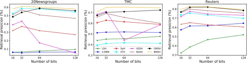
Figure 2: The performance of unsupervised hashing models on three datasets with various numbers of hashing bits.
set to be1×10−3, with a decay rate of 0.96 for every 10000 iterations. The component numberK
and the parameterαin (11) are determined based on the validation set.
Baselines For unsupervised semantic hashing, we compare the proposed GMSH and BMSH with the following models: locality sensitive hashing (LSH), stack restricted boltzmann ma-chines (S-RBM), spectral hashing (SpH), self-taught hashing (STH), variational deep semantic hashing (VDSH) and neural architecture for se-mantic hashing(NASH). For supervised sese-mantic hashing, we also compare GMSH-S and BMSH-S with the following baselines: supervised hashing with kernels (KSH) (Liu et al., 2012), semantic hashing using tags and topic modeling (SHTTM) (Wang et al.,2013), supervised VDSH and super-vised NASH.
Evaluation Metrics For every document from the testing set, we retrieve similar documents from the training set based on the hamming distance be-tween their hashing codes. For each query, 100 closest documents are retrieved, among which the documents sharing the same label as the query are deemed as the relevant results. The ratio between the number of relevant ones and the total number, which is 100, is calculated as the similarity search precision. The averaged value over all testing doc-uments is then reported. The retrieval precisions
under the cases of 16 bits, 32 bits, 64 bits, 128 bits hashing codes are evaluated, respectively.
4.2 Performance Evaluation of Unsupervised Semantic Hashing
ad-Datasets TMC 20Newsgroups Reuters
Method 16bit 32bit 64bit 128bit 16bit 32bit 64bit 128bit 16bit 32bit 64bit 128bit
[image:7.595.82.521.198.328.2]KSH 0.6842 0.7047 0.7175 0.7243 0.5559 0.6103 0.6488 0.6638 0.8376 0.8480 0.8537 0.8620 SHTTM 0.6571 0.6485 0.6893 0.6474 0.3235 0.2357 0.1411 0.1299 0.8520 0.8323 0.8271 0.8150 VDSH-S 0.7887 0.7883 0.7967 0.8018 0.6791 0.7564 0.6850 0.6916 0.9121 0.9337 0.9407 0.9299 NASH-DN-S 0.7946 0.7987 0.8014 0.8139 0.6973 0.8069 0.8213 0.7840 0.9327 0.9380 0.9427 0.9336 GMSH-S 0.7806 0.7929 0.8103 0.8144 0.6972 0.7426 0.7574 0.7690 0.9144 0.9175 0.9414 0.9522 BMSH-S 0.8051 0.8247 0.8340 0.8310 0.7316 0.8144 0.8216 0.8183 0.9350 0.9640 0.9633 0.9590
Table 2: The performances of different supervised hashing models on three datasets under different lengths of hashing codes.
16 15
0 13
14 7
8 12 10
11 19 2
17 1 4
6 3 5
9 18
(a) VDSH-S
17
7 12
13 14
5 4
11 6
19
2 0
3
15
16 10
18
1 9
8
(b) GMSH-S
0
8 19
2
1
6
5
11 17 16
18 13
12 10
14
7 4
3 9
15
[image:7.595.101.257.398.513.2](c) BMSH-S
Figure 3: Visualization of the 32-dimensional document latent semantic embeddings learned by VDSH-S, GMSH-S and MBGMSH-SH-GMSH-S on 20Newsgroups dataset. Each data point in the figure denotes a document, with each color representing one category. The number shown with the color is the ground-true category ID.
Figure 4: The retrieval precisions of GMSH and BMSH on three datasets in both unsupervised and supervised scenarios.
vantages of producing more distinguishable codes with a mixture prior and end-to-end training en-abled by a Bernoulli prior. BMSH integrates the merits of NASH and GMSH, and thus is more suit-able for the hashing task.
Figure 2 shows how retrieval precisions vary with the number of hashing bits on the three datasets. It can be observed that as the number increases from 32 to 128, the retrieval precision-s of moprecision-st previouprecision-s modelprecision-s tend to decreaprecision-se. Thiprecision-s phenomenon is especially obvious for VDSH, in which the precisions on all three datasets drop by a significant margin. This interesting phenomenon has been reported in previous works (Shen et al.,
2018; Chaidaroon and Fang, 2017; Wang et al.,
2013; Liu et al., 2012), and the reason could be overfitting since the model with long hashing codes is more likely to overfitting (Chaidaroon and Fang,2017;Shen et al.,2018). However, it can be seen that our model is more robust to the number of hashing bits. When the number is increased to 64 or 128, the performance of our models is kept almost unchanged. This may be also attributed to the mixture priors imposed in our models, which can regularize the models more effectively.
4.3 Performance Evaluation of Supervised Semantic Hashing
We evaluate the performance of supervised hash-ing in this section. Table 2 shows the perfor-mances of different supervised hashing models on three datasets under different lengths of hashing codes. We observe that all of the VAE-based gen-erative hashing models (i.e VDSH, NASH, GMSH and BMSH) exhibit better performance, demon-strating the effectiveness of generative models on the task of semantic hashing. It can be also seen that BMSH-S achieves the best performance, sug-gesting that the advantages of Bernoulli mixture priors can also be extended to the supervised sce-narios.
K
D 20Newsgroups TMC Reuters
GMSH BMSH GMSH BMSH GMSH BMSH
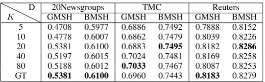
5 0.4708 0.5977 0.6886 0.7492 0.7888 0.8152 10 0.4778 0.6007 0.6862 0.7479 0.8039 0.8226 20 0.5381 0.6100 0.6883 0.7495 0.8182 0.8286 40 0.5197 0.6015 0.7024 0.7481 0.8169 0.8258 80 0.5188 0.6012 0.7033 0.7467 0.8087 0.8253
[image:8.595.164.435.60.144.2]GT 0.5381 0.6100 0.6960 0.7443 0.8183 0.8279
Table 3: Precisions of top 100 retrieved documentswith different numberer of clusters,Kdenotes the number of components, D represents datasets, GT represents the ground truth number of classes for each dataset.
performance gain of the four proposed models, the retrieval precisions of GMSH, BMSH, GMSH-S and BMSH-S using 32-bit hashing codes on the three datasets are plotted together in Figure4. It can be obviously seen that GMSH-S and BMSH-S outperform GMBMSH-SH and BMBMSH-SH by a substantial margin, respectively. This suggests that the pro-posed generative hashing models can also lever-age the label information to improve the hashing codes’ quality.
4.4 Impacts of the Component Number
To investigate the impacts of component number, experiments are conducted for GMSH and BMSH under different values of K. For demonstration convenience, the length of hashing codes is fixed to 32. Table 3 shows the precisions of top 100 retrieved documents when the number of compo-nentsKis set to different values. We can see that the retrieval precisions of the proposed models, e-specially the BMSH, are quite robust to this pa-rameter. For BMSH, the difference between the best and worst precisions on the three datasets are 0.0123, 0.0052 and 0.0134, respectively, which are small comparing to the gains that BMSH has achieved. One exception is the performance of GMSH on 20Newsgroups dataset. However, as seen from Table3, as long as the numberKis not too small, the performance loss is still acceptable. It is worth noting that the worst performance of GMSH on 20Newsgroups is 0.4708, which is still better than VDSH’s 0.4327 as in Table1. For the BMSH model, the performance is stable across all the considered datasets andKvalues.
4.5 Visualization of Learned Embeddings
To understand the performance gains of the pro-posed models better, we visualize the learned rep-resentations of VDSH-S, GMSH-S and BMSH-S on 20Newsgroups dataset. UMAP (McInnes et al.,2018) is used to project the 32-dimensional latent representations into a 2-dimensional space, as shown in Figure3. Each data point in the figure
denotes a document, with each color representing one category. The number shown with the color is the ground truth category ID. It can be observed from Figure 3 (a) and (b) that more embeddings are clustered correctly when the Gaussian mixture prior is used. This confirms the advantages of us-ing mixture priors in the task of hashus-ing. Fur-thermore, it is observed that the latent embeddings learned by BMSH-S can be clustered almost per-fectly. In contrast, many embeddings are found to be clustered incorrectly for the other two models. This observation is consistent with the conjecture that mixture prior and end-to-end training are both useful for semantic hashing.
5 Conclusions
In this paper, deep generative models with mix-ture priors were proposed for the tasks of semantic hashing. We first proposed to use a Gaussian mix-ture prior, instead of the standard Gaussian prior in VAE, to learn the representations of documents. A separate step was then used to cast the con-tinuous latent representations into binary hashing codes. To avoid the requirement of a separate cast-ing step, we further proposed to use the Bernoulli mixture prior, which offers the advantages of both mixture prior and the end-to-end training. Com-paring to strong baselines on three public datasets, the experimental results indicate that the proposed methods using mixture priors outperform existing models by a substantial margin. Particularly, the semantic hashing model with Bernoulli mixture prior (BMSH) achieves state-of-the-art results on all the three datasets considered in this paper.
6 Acknowledgements
References
Yoshua Bengio, Nicholas L´eonard, and Aaron Courville. 2013. Estimating or propagating gradi-ents through stochastic neurons for conditional com-putation.arXiv preprint arXiv:1308.3432.
Samuel R Bowman, Luke Vilnis, Oriol Vinyals, An-drew M Dai, Rafal Jozefowicz, and Samy Bengio. 2015. Generating sentences from a continuous s-pace. arXiv preprint arXiv:1511.06349.
Suthee Chaidaroon, Travis Ebesu, and Yi Fang. 2018. Deep semantic text hashing with weak supervision. SIGIR.
Suthee Chaidaroon and Yi Fang. 2017. Variational deep semantic hashing for text documents. In Pro-ceedings of the 40th International ACM SIGIR Con-ference on Research and Development in Informa-tion Retrieval, pages 75–84. ACM.
Xi Chen, Diederik P Kingma, Tim Salimans, Yan Du-an, Prafulla Dhariwal, John SchulmDu-an, Ilya Sutskev-er, and Pieter Abbeel. 2016. Variational lossy au-toencoder. arXiv preprint arXiv:1611.02731.
Mayur Datar, Nicole Immorlica, Piotr Indyk, and Va-hab S Mirrokni. 2004. Locality-sensitive hashing scheme based on p-stable distributions. In Proceed-ings of the twentieth annual symposium on Compu-tational geometry, pages 253–262. ACM.
Xin Dong, Alon Halevy, Jayant Madhavan, Ema Nemes, and Jun Zhang. 2004. Similarity search for web services. In Proceedings of the Thirtieth international conference on Very large data bases-Volume 30, pages 372–383. VLDB Endowment.
Hao Fu, Chunyuan Li, Xiaodong Liu, Jianfeng Gao, Asli Celikyilmaz, and Lawrence Carin. 2019. Cycli-cal annealing schedule: A simple approach to mit-igating kl vanishing. In Proceedings of the 2019 Conference of the North American Chapter of the Association for Computational Linguistics: Human Language Technologies, Volume 1 (Long and Short Papers), pages 240–250.
Yunchao Gong, Svetlana Lazebnik, Albert Gordo, and Florent Perronnin. 2013. Iterative quantization: A procrustean approach to learning binary codes for large-scale image retrieval. IEEE Transaction-s on Pattern AnalyTransaction-siTransaction-s and Machine Intelligence, 35(12):2916–2929.
Prasoon Goyal, Zhiting Hu, Xiaodan Liang, Chenyu Wang, and Eric P Xing. 2017. Nonparametric vari-ational auto-encoders for hierarchical representation learning. InProceedings of the IEEE International Conference on Computer Vision, pages 5094–5102.
Zhuxi Jiang, Yin Zheng, Huachun Tan, Bangsheng Tang, and Hanning Zhou. 2016. Variational deep embedding: An unsupervised and genera-tive approach to clustering. arXiv preprint arX-iv:1611.05148.
Diederik P Kingma and Jimmy Ba. 2014. Adam: A method for stochastic optimization. arXiv preprint arXiv:1412.6980.
Diederik P Kingma and Max Welling. 2013. Auto-encoding variational bayes. arXiv preprint arX-iv:1312.6114.
Yehuda Koren. 2008. Factorization meets the neigh-borhood: a multifaceted collaborative filtering mod-el. In Proceedings of the 14th ACM SIGKDD in-ternational conference on Knowledge discovery and data mining, pages 426–434. ACM.
Brian Kulis and Trevor Darrell. 2009. Learning to hash with binary reconstructive embeddings. In Ad-vances in neural information processing systems, pages 1042–1050.
Michael S Lew, Nicu Sebe, Chabane Djeraba, and Ramesh Jain. 2006. Content-based multimedia in-formation retrieval: State of the art and challenges.
ACM Transactions on Multimedia Computing, Com-munications, and Applications (TOMM), 2(1):1–19.
Haomiao Liu, Ruiping Wang, Shiguang Shan, and X-ilin Chen. 2016. Deep supervised hashing for fast image retrieval. In Proceedings of the IEEE con-ference on computer vision and pattern recognition, pages 2064–2072.
Wei Liu, Jun Wang, Rongrong Ji, Yu-Gang Jiang, and Shih-Fu Chang. 2012. Supervised hashing with ker-nels. In Computer Vision and Pattern Recognition (CVPR), 2012 IEEE Conference on, pages 2074– 2081. IEEE.
Wei Liu, Jun Wang, Sanjiv Kumar, and Shih-Fu Chang. 2011. Hashing with graphs. InProceedings of the 28th international conference on machine learning (ICML-11), pages 1–8. Citeseer.
Leland McInnes, John Healy, Nathaniel Saul, and Lukas Grossberger. 2018. Umap: Uniform mani-fold approximation and projection. The Journal of Open Source Software, 3(29):861.
Yishu Miao, Lei Yu, and Phil Blunsom. 2016. Neu-ral variational inference for text processing. In In-ternational Conference on Machine Learning, pages 1727–1736.
Dinghan Shen, Qinliang Su, Paidamoyo Chapfuwa, Wenlin Wang, Guoyin Wang, Lawrence Carin, and Ricardo Henao. 2018. Nash: Toward end-to-end neural architecture for generative semantic hashing.
arXiv preprint arXiv:1805.05361.
Fumin Shen, Chunhua Shen, Wei Liu, and Heng Tao Shen. 2015. Supervised discrete hashing. In
Proceedings of the IEEE conference on computer vi-sion and pattern recognition, pages 37–45.
documents. InProceedings of the 30th annual inter-national ACM SIGIR conference on Research and development in information retrieval, pages 825– 826. ACM.
Jingdong Wang, Ting Zhang, Nicu Sebe, Heng Tao Shen, et al. 2018. A survey on learning to hash.
IEEE Transactions on Pattern Analysis and Machine Intelligence, 40(4):769–790.
Jun Wang, Wei Liu, Sanjiv Kumar, and Shih-Fu Chang. 2016. Learning to hash for indexing big dataa sur-vey. Proceedings of the IEEE, 104(1):34–57.
Qifan Wang, Dan Zhang, and Luo Si. 2013. Semantic hashing using tags and topic modeling. In Proceed-ings of the 36th international ACM SIGIR confer-ence on Research and development in information retrieval, pages 213–222. ACM.
Yair Weiss, Antonio Torralba, and Rob Fergus. 2009. Spectral hashing. InAdvances in neural information processing systems, pages 1753–1760.
Jiaming Xu, Peng Wang, Guanhua Tian, Bo Xu, Jun Zhao, Fangyuan Wang, and Hongwei Hao. 2015. Convolutional neural networks for text hashing. In
IJCAI, pages 1369–1375.
Zichao Yang, Zhiting Hu, Ruslan Salakhutdinov, and Taylor Berg-Kirkpatrick. 2017. Improved variation-al autoencoders for text modeling using dilated con-volutions. arXiv preprint arXiv:1702.08139.