Modelling temperature effects on milk production : a study on Holstein cows at a Japanese farm

R E S E A R C H

Open Access

Modelling temperature effects on milk

production: a study on Holstein cows at a

Japanese farm

Machiko Yano

, Hideyasu Shimadzu

and Toshiki Endo

Abstract

Milk yield and its composition vary according to individual cows as well as to a variety of different environment conditions, such as temperature. Previous studies suggest that heat exerts considerable negative effects on milk production and its composition, especially during summer months. We investigate the production and fat composition of milk from individual dairy cows and develop a modelling framework that investigates the effect of temperature by extending a traditional lactation curve model onto a more flexible statistical modelling framework, a generalised additive model (GAM). The GAM simultaneously copes with multiple different conditions (temperature, parity, days of lactation, etc.), and, importantly, their non-linear relationships. Our analysis of retrospective data suggests that individual cows respond differently to heat; cows producing relatively high quantities of milk tend to be particularly sensitive to heat. Our model also suggests that most dairy cows studied fall into three distinct cases that underpin the variation of the milk fat ratio by different mechanisms.

Keywords: Milk production; Milk fat; Heat stress; Lactation curves; Modelling; Test-day data

Background

It has been well recognised that milk yield and its com-position vary according to individual cows as well as to a variety of different environment conditions, such as tem-perature. Previous studies indicate, for example, that heat exerts considerable negative effects on milk production. Extensive efforts have been made to quantify the effect of heat on milk production, investigating such factors as humidity, wind speed, daylight length, and tempera-ture and humidity indices (THIs). The results generally suggest that heat stress results in decreased milk produc-tion (Barash et al. 2001; Bouraoui et al. 2002; West et al. 2003; Bohmanova et al. 2007) and altered composition (Bandaranayaka and Holmes 1976; McDowell et al. 1976; Schneider et al. 1988); since dairy cows prefer a relatively cool atmosphere, these findings are logical.

*Correspondence: hs50@st-andrews.ac.uk

2School of Biology, Centre for Biological Diversity and Scottish Oceans Institute, University of St Andrews, Dyers Brae House, St Andrews, Fife KY16 9TH, UK 3Department of Mathematics, Keio University, 3-14-1 Hiyoshi Kohoku, Yokohama 223-8522, Japan

Full list of author information is available at the end of the article

To investigate the extent to which the variation of milk production and its composition are driven by individual differences as well as differing environment conditions, including temperature effects, a number of modelling attempts have been undertaken. There are two major modelling streams: lactation curve models (Wood 1976) and random regression test-day models (Schaeffer 2004). The most challenging aspect of modelling is construct-ing a flexible model that copes with the non-linear nature of milk production and the individual differences in dairy cows; the actual functional relationships are far more complex than simple linear relationships. In this respect, the lactation curve model is a non-linear model, but it is not flexible enough to deal simultaneously with indi-vidual differences and other multiple differing conditions. On the other hand, the random regression test-day model is capable of describing both individual differences and other multiple conditions, but it often restricts its atten-tion to particular linear relaatten-tionships.

In this study, we aim to develop a flexible mod-elling framework that utilises the previous two modmod-elling approaches. Our modelling framework is built directly on the lactation curve model. We extend this traditional

model onto a well-known statistical modelling frame-work: the generalised additive model (GAM; Hastie and Tibshirani 1990). The GAM provides enhanced modelling flexibility that copes with both multiple differing condi-tions and individual differences, and is therefore effective in modelling non-linear relationships.

We model the effect of temperature on the yield and fat composition of milk produced by individual cows. Our analysis of retrospective data suggests that cows produc-ing high quantities of milk are sensitive to heat and tend to decrease their milk production as the ambient tempera-ture increases. Additionally, most dairy cows studied here fall into three distinct cases that underpin the variation of milk fat ratios by different mechanisms.

Results Models

The composition of milk varies according to individual cows as well as to different environment conditions. We investigate two major components of milk production: (i) the milk yield, y, and (ii) the milk fat ratio, z, as recorded in the test-day data (see Materials and methods). To investigate the extent to which the variation of these components is driven by different factors, a number of modelling attempts has been undertaken. These have utilised lactation curves (Allore et al. 1997; Barash et al. 2001; Bouraoui et al. 2002; Wood 1976) and test-day data modelling (Bignardi et al. 2012; Kettunen et al. 2000; Schaeffer 2004), independently fitting a single model to each component. In doing so, however, these studies have incorrectly made a model assumption of the error struc-ture, which may lead to biased inference. We can clearly see this from the definition of the milk fat ratio:

z= z

y, (1)

wherezis the amount of milk fat. Here, the milk fat ratio,

z, is a function of the milk yield,y, and the milk fat yield,

z. Accordingly, the variation of the milk fat ratio originates from that of the milk yield as well as the milk fat yield. In other words, the milk fat ratio is derived from the milk yield or the milk fat; they are, therefore, always dependent. We here propose a simple modelling approach that properly copes with relationship (1). Our model is also related with traditional lactation curve models as well as random regression test-day models (see Discussion). We model the milk yield,yit, and the milk fat yield,zit, (not the

milk fat ratio) from thei-th cow at timetin the natural logarithmic scale as

log(yit) = αi+aiwt+

j

sj(xjt)+εit, (2)

log(zit) = βi+biwt+

j

tj(xjt)+ξit, (3)

where εit andξit are respectively independent Gaussian

noise with variance σ_ε2_i and σ_ξ2_i between cows, i. The functions here,sj(·)andtj(·), are smoothing spline

func-tions whose functional form can differ among the covari-ates,xj’s such as parity, days of lactation, calving month,

amount of concentrate feed, and day length: the various calving conditions. Some of these can be individual-dependent, for which the notation should bexijt, but we

drop the subscriptifor simplification.

The model here assumes a linear relationship with the daily maximum temperature,wt. This can be regarded as

a linear approximation of the smooth non-linear function

s(wt) or t(wt). Such an approximation is able to

cap-ture the temperacap-ture effect in a parsimonious way; the effect is now expressed by only one parameter, the tem-perature coefficientaiorbi that varies among individual

cows,i. A negative value indicates decreased milk or milk fat production as the maximum temperature increases; a positive value indicates the opposite situation, increased milk or milk fat production, because of an increase of the maximum temperature.

The parametersα_i,ai,σε2iand the smooth functionsjin

Equation (2) are estimable from the data under the gener-alised additive modelling (GAM; Wood 2006) framework (see Materials and methods). In contrast, the parameters βi,bi,σξ2iand the smooth functiontjin Equation (3)

can-not be directly estimated from our test-day data since no records of milk fat, zit, are actually available.

How-ever, by noting the relationship (Equation (1)), they can be estimated through the milk fat ratio,z, recorded in the test-day data. Since we know relationship (1), the milk fat ratio in the natural logarithmic scale can be described as

log(z_it) = log(zit)−log(yit)

= βi+biwt+

j

tj(xjt)+ξit−log(yit), (4)

where log(yit) is an offset term andξit is an error term.

We can then fit the models (Equations (2) and (3)) using the relationship given in Equation (4). A disregard for the offset term when fitting the model is equivalent to fitting a single independent model to the milk fat ratio. In doing so, if models (2) and (3) are correct, an inappropriate error structure is introduced, by minimising the sum of squared residuals _it(ξ_it −log(yit))2. As Equation (4) shows,

the correct procedure in parameter estimation should be to minimise_itξ_it2, instead.

Temperature effects on individual dairy cows

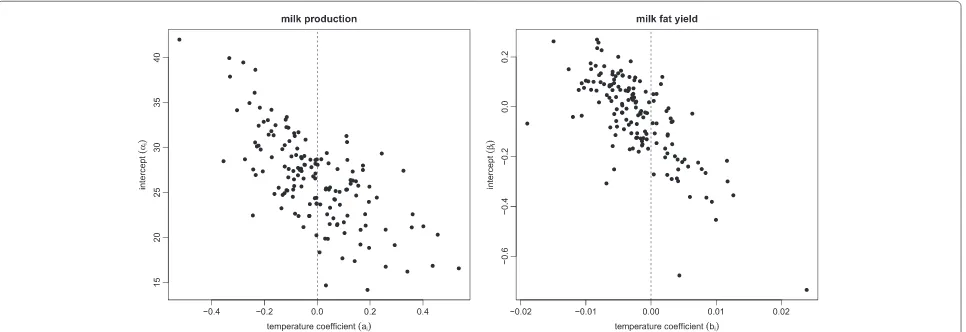
Temperature has a greater influence on cows that produce relatively high amounts of milk and fat content. Figure 1 shows the scatter plots of the intercept of milk produc-tion,αi, (left) and the milk fat yield,βi, (right) against their

Figure 1Plots of the constants for milk production and the milk fat yield against the respective temperature coefficients.The superposed dashed line separates individual cows into groups according to whether their temperature coefficient is positive or negative. This negative correlation between the constant and the temperature coefficient suggests that relatively highly productive cows are sensitive to heat.

temperature coefficient indicates decreased milk or milk fat production as the maximum temperature increases. A positive one implies increased milk or milk fat production due to an increase in the maximum temperature. Each plot shows a clear negative correlation, indicating that the cows that are relatively highly productive tend to be more sensitive to heat and may decrease their productivity when the temperature increases. Our results support the findings of previous studies (Johnston 1958; Bianca 1965; Barash et al. 2001) as well. They report that highly produc-tive cows tend to have a relaproduc-tively high body temperature, and are therefore more sensitive to heat.

Variation of the milk fat ratio according to temperature

Many farms use the milk fat ratio as an indicator of milk quality. We rewrite the milk fat ratio,z, from Equation (4) as

log(z_it)=γi+riwt+

j

uj(xjt)+ηit,

whereγi = βi−αi,ri= bi−ai,uj(xjt) =tj(xjt)−sj(xjt)

andηit = ξit −εit. Figure 2 shows the variation of the

milk fat ratio according to heat; the interceptγiis plotted

against the temperature coefficient,ri. The plot also shows

a negative correlation, indicating that temperature has a greater effect on the cows that produce milk with a higher milk fat ratio. A negative temperature coefficient indicates a decrease in the milk fat ratio, while a positive one indi-cates an increase in the milk fat ratio when the maximum temperature increases.

We have found that there are three main scenarios responsible for a decrease in the milk fat ratio: (1) a decrease in milk fat and an increase in milk production (Case 1,bi < 0 < ai); (2) an increase in milk fat and

milk production, but a relatively faster increase in the lat-ter (Case 2,ai > bi > 0); and (3) a decrease in milk fat

and milk production, but a relatively faster decrease in the former (Case 3,bi <ai <0). The reverse three scenarios

are responsible for an increase in the milk fat ratio (Case 4,

ai<0<bi; Case 5,ai<bi<0; and Case 6,bi>ai>0).

Figure 3 illustrates how individual cows fall into these six cases, by plotting the temperature coefficient of the milk fat against the temperature coefficient of the milk yield. The solid line (bi=ai) separates the individual cows

into two categories according to whether their milk fat ratio increases (left) or decreases (right) as the maximum temperature increases. Clearly, most individual cows fall into one of three cases: Case 1, Case 2, and Case 5. This underscores the fact that for some dairy cows, heat stress leads to an increase in the milk fat ratio. However, few of these cases are caused by an increase in the milk fat yield (Case 4); most are the result of a relatively faster decrease in milk production (Case 5).

Response curves of milk production and milk fat yield

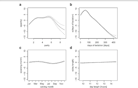
Our model also describes how the milk content responds to different calving conditions, such as parity, days of lac-tation, calving month, and day length. Figure 4 shows the response curve of milk production to each calving con-dition. The amount of concentrate feed is excluded, as it is dependent upon the amount of milk produced by each cow.

Figure 2Plot of the constant for the milk fat ratio against the temperature coefficient.The superposed dashed line separates individual cows into groups according to whether their temperature coefficient is positive or negative. This negative correlation between the constant and the temperature coefficient suggests that relatively highly productive cows are sensitive to heat.

Figure 3Scatter plot of the temperature coefficients from milk production (ai) and milk fat (bi).There are six possible scenarios (cases)

causing a decrease or an increase in the milk fat ratio. These cases are distinguished by the combination of the signs of the temperature coefficients

a

b

c

d

Figure 4The estimated response curves of milk production,sj.Each panel illustrates how the milk yield responds to different calving or

environment factors:a)parity;b)days of lactation;c)calving month; andd)day length. The dashed lines are point-wise twice standard-error bands.

according to region. For instance, the lactation curve of European breeds becomes practically linear or has a flat peak (Madalena et al. 1979) in tropical regions; for British herds, the maximum production normally occurs in week five of lactation (Wood 1969).

Milk production also varies according to parity and calv-ing month. Production peaks around the fourth lactation (Figure 4a). In comparison with days of lactation and par-ity, calving month had a smaller effect on the lactation curve (Figure 4c). As Barash et al. (2001) report, the lowest production occurs in summer, and the highest in winter. We have also investigated the photoperiod effect, that is, varying daylight length. Figure 4d shows a slight increase trend according to longer day length, but its influence is muted in comparison with parity and days of lactation.

Figure 5 shows the response of the milk fat compo-nent to the conditions of parity, days of lactation, calving month, the amount of concentrate feed, and day length. The responses to parity (Figure 5a) and calving month (Figure 5c) are similar to those shown by milk produc-tion; the response curve to parity also shows a peak at the second to fifth lactation. As Barash et al. (2001) report, calving month has a smaller effect on the milk fat com-ponent, with the lowest milk fat yield occurring during summer. The response of the milk fat component to days

of lactation (Figure 5b) differs most from that of milk production. The fat component is richest at the start of lactation, falls sharply until around 60 days, and thereafter continues to decrease, although relatively more slowly than in the first 60 days. The effect of daylight length (Figure 5d) also shows an almost flat trend. The response curve to concentrate feed increases gradually, indicating that higher feed intake triggers increased production of milk fat.

Discussion

Relation to previous studies

Lactation curves

Our model is a direct extension of traditional lactation curve models. The early study of the lactation curve can be found in Gaines (1927) and Vujicic and Bacic (1961) and then Wood (1976) refine the traditional lactation curve model. There have been extensive studies undertaken since then (Gnanasakthy and Morant 1990; Goodall 1983; Lannox et al. 1992; Wood 1969; Wood 1972; Wood 1976). Wood (1976) describes milk yield in a non-linear manner:

a

b

c

e

d

Figure 5The estimated response curves of the milk fat yield,tj, with point-wise twice standard-error bands.Each panel illustrates how the

wherea,b, andcare parameters to be estimated andηt

is an error term. Note that this parametric model is a function of the timetsince calving.

The non-linear model shown in Equation (5) gener-ally works well, but only takes into account the time since calving. Many model extensions have been proposed that allow the parameters to vary according to different conditions, such as seasonal variation (Gnanasakthy and Morant 1990; Goodall 1983; Wood 1972; Wood 1976) regional variation (Gnanasakthy and Morant 1990), and livestock diet (Lannox et al. 1992).

Our present model provides a more flexible framework, which encompasses the Wood model and its extensions as special cases. For example, taking a natural logarithm of Equation (5), it can be written as

log(yt)=log(a)+blog(t)−ct+εt,

whereε_t = log(η_t). By comparing this with Equation (2), and rewriting the time since calving ast=xjt, we obtain

log(a) = αi+aiwt+

j=j sj(xjt),

blog(t)−ct = sj(xjt).

Clearly, our model has extended the lactation curve model, re-parameterising parameters a,b, and c in a more flexible manner. This re-parametrisation provides enhanced modelling flexibility. First, the constant term, log(a), is able to cope with the variation originating from factors such as temperature and different calving con-ditions. Second, the traditional lactation curve is now described as a nonparametric function,sj, the shape of

which can be estimated from the data.

Random regression test-day models

Random regression models for test-day data have become increasingly common in animal breeding research. Our model is also related to this modelling approach. A large number of applications can be found in the analysis of the genetic evaluation of dairy cows; see Schaeffer (2004) for a concise review of the model in this area. The basic form of the model consists of three parts: random effects, fixed effects, and an error term, and these terms are accordingly described in the model form as

log(yit)=

j

Aijzijt+

j

fj(xjt)+εit, (6)

for the milk yieldyit of thei-th individual at time t, for

example. On the right-hand side of the model (Equation (6)), the first term, random effects, has a linear form, and each parameterAijis assumed to be normally distributed

with mean zero (EAij

= 0) and a constant variance (VarAij

= σ2

Aj); the second term, fixed effects fj(xjt)

(including a constant term f1(1)), can have a linear or

non-linear form (but is often linear); and the error term εit is the Gaussian error with mean zero, but it is not

identical; the variance of the error differs in individ-ual cows (Var [εit] = σε2i), but they are uncorrelated

(Cov [εit,εit] = 0 for i = i). In the context of

ran-dom regression test-day models, the ranran-dom effect often represents two effects, genetic and permanent environ-mental effects. The construction of the model also relies on its variance-covariance structure, for which a variety of structures are available.

Takingzi1t = 1,zi2t = wt (accordingly Ai1 = αi and Ai2=ai) andfj=sj, it is clear that the random regression

test-day model becomes almost identical to our model (Equation (2)) except for the fact that parameter Aij is

assumed to be normally distributed; our model does not assume any distributions for the parameters, but instead estimates them for each individual cow as αˆi or

ˆ

ai(i=1, 2,. . ., 153). They are fixed effects, in other words.

This is the essential difference between the two models. However, it is interesting to note that this makes little difference in the estimation, although it does make a dif-ference in the prediction. For example, the random regres-sion test-day models cannot distinguish individual cows by parameterAij as we have done and discussed in the

Results section. In contrast, our model cannot give a pre-diction for absent cows in the data because the individual-dependent parameters are inestimable for unobserved cows. There is no single answer of the question of which model is actually ‘correct’; the choice is largely depen-dent on the research question. If it aims to predict for a general population of cows regardless of whether they are observed or not, then the random regression test-day model would be more appropriate, but if it intends to distinguish individual cows, as we have discussed, then our model becomes a more suitable candidate.

Effects of temperature on individual dairy cows

Our present results highlight the importance of investi-gating individual differences. Although it is beyond our present study, it is likely that such differences, even within the same species, are somehow related to genetic differ-ences. A number of studies on Holsteins have investigated the interaction between genotypes and environmental conditions. Ravagnolo et al. (2000) conclude that consid-erable genetic variation exists within the Holstein breed. Our model is, however, still able to cope with such genetic differences indirectly as a constant effect, allowing the intercept to differ between individual cows, even though we have no genetic data to characterise individuals. This is the virtue of our modelling approach.

Management indications

resembles the reciprocal of milk production, as shown in Equation (1). This fact vindicates an empirical finding by Wood (1976). Of course, there is a variety of choices of which indicator to use for management, and it is abso-lutely the farm’s choice. If the milk fat ratio tends to be preferable, the six different scenarios leading to a variation of the milk fat ratio provide useful indications for manage-ment planning strategies. Although managemanage-ment actions to reduce the negative effects of heat cannot be applied to each individual within a large production system (André et al. 2011), our present analysis highlights only six dif-ferent required treatment strategies. Further, these may be reduced to the three major cases shown in Figure 3. Appropriate management action can be taken regarding feed composition and the prioritised allocation of cows in the barn. For Case 2, in which the production of milk and milk fat increase, no special treatment is actually required despite a decrease in the milk fat ratio. The reason for this is the faster increase of milk production compared to that of milk fat yield. For Case 5, cows are strongly affected by heat, but the milk fat ratio increases. The decreased production of milk and milk fat may be offset by allocating the cows as cool a space as possible and provid-ing them with easily digestible and high-calorie feed. For Case 1, the decreased production of milk fat may be offset by providing cows with a fat-productive feed.

Concluding remarks

We have presented a modelling framework for milk pro-duction and its fat component from individual dairy cows by extending both the traditional lactation curve model (Wood 1976) and random regression test-day data models (Schaeffer 2004) onto a more flexible statistical mod-elling framework, GAM. The GAM allows simultaneous modelling of various calving conditions in an appropriate non-linear structure. Our model has shown clear evidence that cows producing high quantities of milk are sensitive to heat and tend to decrease their milk production as the temperature increases. However, some individuals rela-tively increase their milk production as the temperature increases.

Our analysis has suggested that the milk fat ratio is dependent upon and driven by the variation of milk and milk fat production according to heat. We have identi-fied six distinct scenarios that underpin an increase or a decrease in the milk fat ratio. Our results indicate that efficient managing strategies are required for each group; varying the feed composition may be effective.

Given the retrospective nature of our study data, we are unable to determine whether the variation in milk pro-duction is directly driven by high temperature itself or whether a high temperature indirectly triggers poor feed supply. Nevertheless, by revealing different scenarios lead-ing to a variation in the milk fat ratio, our model provides

useful indications for management planning strategies. The model can also be applied to milk components such as the protein yield and protein ratio (also a common indi-cator of milk quality). Moreover, providing that sufficient data are available, the model can be used to predict future milk production and composition.

Materials and methods Data

Throughout this paper, we focus on two data sets: (i) the test-day data and (ii) the environment data, which include daily maximum temperature records and daylight length for the studying period (1989–1998) at Jiyu Gakuen Nasu Farm (36°56N, 139°58E) in Tochigi Prefecture, which has the second-largest dairy cow population in Japan.

The test-day data for individual dairy cows comprise six items, namely, milk yield, milk fat ratio (the amount of milk fat is not given), parity, days of lactation, calv-ing month, and amount of concentrate feed (see Table 1 for the summary statistics). The test is undertaken and reported every month by the Livestock Improvement Association of Japan Inc.

We have selected 153 lactating Holstein cows from the farm for which test-day data are available over a mini-mum of twelve months. The number of data points vary according to individual cows; they comprise between 12 and 65 observations in total for each. Those data all are used to estimate the parameters of the models. The cows are housed in a covered tie stall barn with no cooling sys-tem for 20 hours per day. Except when raining, the cows are generally kept outside from 10 a.m. to 2 p.m. All of the cows are milked and fed twice daily, at 5 a.m. and 4:30 p.m. Although the amount and composition of feeds vary depending on cows’ condition, a combination of for-ages and concentrate feed consisting of carbohydrate and protein (maize and oats (32%), wheat and rice bran, and soy (25%), oil cake of soy and coleseed (10%), and others (33%)) is supplied.

To investigate the effect of temperature, we use the daily maximum temperature recorded on the day of test-ing by ustest-ing a maximum-minimum thermometer in an

Table 1 Summary statistics of the test-day data

Min Median Mean Max

Milk production [kg] 3.20 26.20 26.33 53.00

Milk fat ratio [%] 2.20 3.80 — 7.90

Parity 1.00 2.00 2.58 9.00

Calving month 1.00 8.00 7.03 12.00

Days of lactation 1.00 173.00 176.10 430.00

Amount of concentrate feed [kg] 1.00 10.00 9.52 20.00

instrument shelter located 20 metres from the dairy barn. The monthly variation shows a typical unimodal trend, with a peak of around 30°C during summer and a trough of around 7°C during winter (Figure 6a). The greatest dif-ference, around 23 degrees, occurs between January and July.

The daylight length of each test day is calculated as follows. Given a solar location on the celestial sphere; that is, the declination and right ascension (δ(d),α(d)) of a particular date and time, sunrise and sunset times,

d, at a geological location (λ,ψ) on the Earth satisfy the following equation (Nagasawa 1999):

sinδ(d)sinψ+cosδ(d)cosψcost(d)−sink(d)=0, wheret(d) = 0(d)+λ−α(d) is the solar hour angle andk(d) is the solar elevation. The monthly variation of the daylight length of test days is illustrated in Figure 6b; it varies within a five-hour difference (between about 9.5 to 14.5 hours) over a year, which is a narrower variation in comparison with other higher-latitude countries. The monthly variations also show a typical unimodal trend, with a peak at June and a trough at December, the sum-mer and winter solstices. Note that this peak and trough do not coincide with those of the maximum temperature (Figure 6a).

Parameter estimation

For ease of exposition, we describe the parameter estimation procedure, taking the model of milk yield (Equation (2)) as an example. We rewrite the model using vector notation as

log(y)=α+aw+

j sj+ε,

wherey = (y11,y12,. . .,y1T1,y21,. . .,y31,. . .,y153T153), for example. The parameters to be estimated here areα,a,

and the smooth functionsj. In particular, eachsjis mod-elled by a smooth spline function (Hastie and Tibshirani 1990). We also assume the heteroscedasticity ofε, which means that the errorεitis not identical but uncorrelated

between individual cows; the covariance matrix of the error,, is then given as

=Eεε=

⎛ ⎜ ⎜ ⎜ ⎜ ⎜ ⎜ ⎜ ⎜ ⎝

σ2

1I1

0

σ2 2I2

. ..

0

153I153 ⎞ ⎟ ⎟ ⎟ ⎟ ⎟ ⎟ ⎟ ⎟ ⎠

, (7)

whereIiis an identity matrix whose diagonal elements are all 1. Note that the variancesσ_i2, (i = 1, 2,. . ., 153) are now also parameters to be estimated. As to the covari-ance matrix structure here (Equation (7)), it specifically assumes statistical independence within cows over time; no temporal correlations, in other words, are assumed which can be relaxed for future model extension.

To estimate those parameters and smooth functions, we minimise the weighted least squared

ε−1_{ε−→min (8)}

under the GAM framework, recalling thatε = log(y)− (α + aw+ _jsj). Here, the diagonal elements of the inverse matrix are reciprocal of each variance,−1_ii = 1/σ_i2. However, to estimate the variance components, we have to explicitly model the variance heterogeneity. It is known that the normalised squared residual follows the chi-squared distribution with 1 degree of freedom,

a b

ε2

it/σi2 ∼ χ12. As the the chi-squared random variable is twice a gamma variable with 1/2 degree of freedom, we fit a simple generalised linear model (GLM; McCullagh and Nelder 1989) with the gamma distribution,(1/2, 2), as

logEε2_it=log(σ_i2)=τ_i. (9)

The estimate of variance is then given asσˆ_i2=exp(τˆ_i). The estimation algorithm employed is summarised as follows.

1. Apply Equation (8) withσ2

i =1;

2. Repeat steps 3 to 4 until the estimates stop changing;

3. Estimateτiby Equation (9);

4. Apply Equation (8) with weight σ2

i = ˆσi2=exp(τˆi).

We have conducted the analysis and modelling tasks by a statistical computing language R (R Core Team 2013).

Model diagnostics

Our models (2) and (4) assume a linear relationship between the maximum temperature and each of the milk production and the milk fat as a simple approximation. We inspect whether the assumption made is reasonably appropriate by plotting partial residuals which are defined as

ˆ

εw

it = log(yit)−

j

ˆ

sj(xjt)= ˆαi+ ˆaiwt+ ˆεit,

ˆ

ξw

it = log(zit)−

j

ˆ

tj(xjt)= ˆβi+ ˆbiwt+ ˆξit.

Additional files 1 and 2 respectively show the partial resid-ual plots of the milk production,εˆ_itw, and of the milk fat,

ˆ

ξw

it, for each cow. We have interpreted these plots as that

the majority of the cows, although there are of course some exceptions, appear to have a linear relationship with the maximum temperature rather than non-linear of a particular form.

To assess the goodness of fit of our models, we plot the fitted values of the milk production (Additional file 3) and of the milk fat (Additional file 4) in the natural log scale for each cow, along with the observations. The superposed red line in each panel represents the fitted values. Based on this visual assessment, we regard that while our model is not perfect, it reasonably represents the data observed. Although there are some observations lying slightly away from the fitted value, we for now leave them for further investigations in the future.

Additional files

Additional file 1: The partial residual plots of the milk production,

ˆ

εwit, for each cow.

Additional file 2: The partial residual plots of the milk fat,ξˆw_it, for each cow.

Additional file 3: The fitted values of the milk production in the natural log scale for each cow, along with the observations.The superposed red line in each panel represents the fitted values.

Additional file 4: The fitted values of the milk fat in the natural log scale for each cow, along with the observations.The superposed red line in each panel represents the fitted values.

Competing interests

The authors declare that they have no competing interests.

Authors’ contributions

MY and TE carried out the data entry and its manipulation. MY and HS undertook the data analysis and modelling, and drafted the manuscript. TE participated in the analysis and helped drafting the manuscript. All authors read and approved the final manuscript.

Acknowledgements

The authors are grateful to the late Izumi Yamaguchi for his tremendous effort and work during 57 years of meteorological observation. The maximum temperature records used in our study are obtained from his records. Our sincerest thanks also go to Yo Yamaguchi and Jiyu Gakuen Nasu Farm for allowing us to use the data sets, and to the anonymous reviewers for their valuable comments.

Author details

1_{Jiyu Gakuen College, 1-8-15 Gakuen-cho, Higashikurume-shi, Tokyo} 203-8521, Japan.2_{School of Biology, Centre for Biological Diversity and} Scottish Oceans Institute, University of St Andrews, Dyers Brae House, St Andrews, Fife KY16 9TH, UK.3_{Department of Mathematics, Keio University,} 3-14-1 Hiyoshi Kohoku, Yokohama 223-8522, Japan.

Received: 10 April 2013 Accepted: 30 January 2014 Published: 7 March 2014

References

Allore HG, Oltenacu PA, Erb HN (1997) Effects of season, herd size, and geographic region on the composition and quality of milk in the northeast. J Dairy Sci 80: 340–349

André G, Engel B, Berentsen PBM, Vellinga TV, Oude Lansink AGJM (2011) Quantifying the effect of heat stress on daily milk yield and monitoring dynamic changes using an adaptive dynamic model. J Dairy Sci 94: 4502–4513

Bandaranayaka DD, Holmes CW (1976) Changes in the composition of milk and rumen contents in cows exposed to a high ambient temperature with controlled feeding. Trop Anim Health Prod 8: 38–46

Barash H, Silanikove N, Shamay A, Ezra E (2001) Interrelationships among ambient temperature, day length and milk yield in dairy cows under a Mediterranean climate. J Dairy Sci 84: 2314–2320

Bianca W (1965) Reviews of the progress of dairy science. Section A. Physiology. Cattle in a hot environment. J Dairy Res 32: 291–345 Bignardi A, Faro LE, Santana M, Rosa G, Cardoso V, Machado P, Albuquerque L

(2012) Bayesian analysis of random regression models using B-splines to model test-day milk yield of Holstein cattle in Brazil. Livest Sci 150: 401–406 Bohmanova J, Misztal I, Cole JB (2007) Temperature-humidity indices as

indicators of milk production losses due to heat stress. J Dairy Sci 90: 1947–1956

Bouraoui R, Lahmar M, Majdoub A, Djemali M, Belyea R (2002) The relationship of temperature-humidity index with milk production of dairy cows in a Mediterranean climate. Anim Res 51: 479–491

Gnanasakthy A, Morant SV (1990) A parsimonious model of seasonal and regional variation in the yield of milk, fat, protein and lactose in dairy cows. Anim Prod 50: 583–584

Goodall EA (1983) An analysis of seasonality of milk production. Anim Sci 36: 69–72

Hastie TJ, Tibshirani RJ (1990) Generalized additive models. Chapman & Hall/CRC, Florida

Johnston JE (1958) The effects of high temperatures on milk production. J Heredity 49: 65–68

Kettunen A, Mäntysaari EA, Pösö J (2000) Estimation of genetic parameters for daily milk yield of primiparous ayrshire cows by random regression test-day models. Livest Prod Sci 66(3): 251–261

Lannox SD, Goddal EA, Mayne CS (1992) A mathematical model of the lactation curve of the dairy cow to incorporate metabolizable energy intake. J R Stat Soc: Ser D 41: 285–293

Madalena FE, Martinez ML, Freitas AF (1979) Lactation curves of

Holstein-Friesian and Holstein-Friesian×gir cows. Anim Prod 29: 101–107 McCullagh P, Nelder J (1989) Generalized Linear Models. 2nd Edition.

Chapman and Hall/CRC, Florida

McDowell RE, Hooven NW, Camoens JK (1976) Effect of climate on performance of Holsteins in first lactation. J Dairy Sci 59: 965–971 Nagasawa K (1999) Computations of Sunrise and Sunset. Chijin Shokan, Tokyo R Core Team (2013) R: a language and environment for statistical computing. R

Foundation for Statistical Computing, Vienna. ISBN 3-900051-07-0 Ravagnolo O, Miszal I, Hoogenboom G (2000) Genetic component of heat

stress in dairy cattle, development of heat index function. J Dairy Sci 83: 2120–2125

Schaeffer LR (2004) Application of random regression models in animal breeding. Livest Prod Sci 86: 35–45

Schneider PL, Beede DK, Wilcox CJ (1988) Nyctherohemeral patterns of acid-base status, mineral concentrations and digestive function of lactating cows in natural or chamber heat stress environments. J Anim Sci 66: 112–125

Vujicic I, Bacic B (1961) New equation of the lactation curve, Vol. 5. Cited by Wood (1969)

West JW, Mullinix BG, Bernard JK (2003) Effects of hot, humid weather on milk temperature, dry matter intake, and milk yield of lactating dairy cows. J Dairy Sci 86: 232–242

Wood PDP (1969) Factors affecting the shape of the lactation curve in cattle. Anim Prod 11: 307–316

Wood, PDP (1972) A note on seasonal fluctuation in milk production. Anim Prod 15: 89–92

Wood PDP (1976) Algebraic models of the lactation curves for milk, fat and protein production, with estimates of seasonal variation. Anim Prod 22: 35–40

Wood SN (2006) Generalized additive models: an introduction with R. Chapman & Hall/CRC, Florida

doi:10.1186/2193-1801-3-129

Cite this article as:Yanoet al.:Modelling temperature effects on milk production: a study on Holstein cows at a Japanese farm.SpringerPlus 20143:129.

Submit your manuscript to a

journal and benefi t from:

7Convenient online submission

7Rigorous peer review

7Immediate publication on acceptance

7Open access: articles freely available online

7High visibility within the fi eld

7Retaining the copyright to your article