Linear and nonlinear optical properties of silica aerogel

(1)

LINEAR AND NONLINEAR OPTICAL PROPERTIES OF

SILICA AEROGEL

Adam Colin Fleming

A Thesis Submitted for the Degree of PhD

at the

University of St Andrews

2019

Full metadata for this item is available in

St Andrews Research Repository

at:

http://research-repository.st-andrews.ac.uk/

Please use this identifier to cite or link to this item:

http://hdl.handle.net/10023/18557

(2)

Linear and Nonlinear Optical Properties of

Silica Aerogel

Adam Colin Fleming

This thesis is submitted in partial fulfilment for the degree of

D

octor of

P

hilosophy

at the

U

niversity of

S

t

A

ndrews

School of Physics and Astronomy

University of St Andrews

KY16 9SS

https://synthopt.wp.st-andrews.ac.uk

(3)

Abstract

Scattering media have traditionally been seen as a hindrance to the controlled transport of light through media, creating the familiar speckle pattern. However such matter does not cause the loss of information but instead performs a highly complex deterministic operation on the incoming flux. Through sculpting the properties of the incoming wavefront, we can unlock the hidden characteristics of these media, affording us far more degrees of freedom than that which is available to us in traditional ballistic optics.

These additional degrees of freedom have allowed for the creation of compact sophisticated optical devices based only on the deterministic nature of light scattering. Such devices include diffraction-limit-beating lenses, polarimeters, spectrometers, and some which can transmit entire images through a scattering substance.

Additional degrees of freedom would allow for the creation of even more powerful devices, in new working regimes. In particular, the application of related techniques where the scattering material is actively modified is limited.

This thesis is concerned with the use of optothermal nonlinearity in random media as a way to provide an additional degree of control over light which scatters through it. Specifically, we are concerned with silica aerogel as a platform for this study.

Silica aerogel is a lightweight skeletal structure of silica fibrils, which results in a material which is up to 99.98 % by volume. This material exhibits a unique cocktail of properties of use such as near unitary refractive index, an order of magnitude lower thermal conductivity, and high optothermal nonlinearity. The latter two of these properties allow for the creation of localised steep thermal gradients, proportionally affecting the low refractive index significantly. Additionally through differing fabrication steps, the opacity, and as a result, we can adjust the scattering strength.

In line with the development of light deterministic light scattering techniques in linear media, we develop through the use of pump-probe setups, a framework for the development of a similar line of techniques in nonlinear scattering media. We show that we can reversibly control the far-field propagation of light in weakly scattering silica aerogel. Following this, we show that nonlinear perturbation can be used to extend and modify the optical memory effect, where slight adjustments in scattering direction maintain the overall correlation of the scattered profile. Finally, we measure the nonlinear transmission matrix, a complete description of how any wavefront would pass through at a particular point in a scattering media, and how that scattering can be modified through the application of an optothermal nonlinearity.

(4)

Candidate’s declarations:

I, Adam Colin Fleming, do hereby certify that this thesis, submitted for the degree of PhD, which is approximately 50,000 words in length, has been written by me, and that it is the record of work carried out by me, or principally by myself in collaboration with others as acknowledged, and that it has not been submitted in any previous application for any degree. I was admitted as a research student at the University of St Andrews in September 2015. I received funding from an organisation or institution and have acknowledged the funder(s) in the full text of my thesis.

Date Signature of candidate

Supervisor’s declaration:

I hereby certify that the candidate has fulfilled the conditions of the Resolution and Regulations appropriate for the degree of PhD in the University of St Andrews and that the candidate is qualified to submit this thesis in application for that degree.

(5)

Permission for publication:

In submitting this thesis to the University of St Andrews we understand that we are giving permis-sion for it to be made available for use in accordance with the regulations of the University Library for the time being in force, subject to any copyright vested in the work not being affected thereby. We also understand, unless exempt by an award of an embargo as requested below, that the title and the abstract will be published, and that a copy of the work may be made and supplied to any bona fide library or research worker, that this thesis will be electronically accessible for personal or research use and that the library has the right to migrate this thesis into new electronic forms as required to ensure continued access to the thesis.

I, Adam Colin Fleming, confirm that my thesis does not contain any third-party material that requires copyright clearance.

The following is an agreed request by candidate and supervisor regarding the publication of this thesis:

PRINTED COPY

No embargo on print copy

ELECTRONIC COPY

No embargo on electronic copy

(6)

Underpinning Research Data or Digital Outputs

Candidate’s declaration

I, Adam Colin Fleming, understand that by declaring that I have original research data or digital outputs, I should make every effort in meeting the University’s and research funders’ requirements on the deposit and sharing of research data or research digital outputs.

Permission for publication of underpinning research data or digital outputs

We understand that for any original research data or digital outputs which are deposited, we are giving permission for them to be made available for use in accordance with the requirements of the University and research funders, for the time being in force.

We also understand that the title and the description will be published, and that the underpinning research data or digital outputs will be electronically accessible for use in accordance with the license specified at the point of deposit, unless exempt by award of an embargo as requested below.

The following is an agreed request by candidate and supervisor regarding the publication of underpinning research data or digital outputs:

No embargo on underpinning research data or digital outputs.

(7)

Acknowledgements

I have had the pleasure to work with a great many wonderful people during my time as a researcher in the Synthetic Optics Group. Primary thanks go, Andrea Di Falco, my supervisor. From being my first-year undergraduate tutor to taking me under his wing for a series of undergraduate projects, followed by a masters project, and finally my PhD, I would not be the researcher I am today without him. Also for letting me travel to far too many pool and snooker competitions.

To all the members of the Synthetic Optics Group both past and present: James Burch, Xin Li, Ranjeet Kumar, Usenobong ’Benjamin’ Akpan, Alasdair Fikouras, Aline Heyerick, Blair Kirkpatrick, Peter Reader-Harris, Michiel Samuels, Nedyalka Panova, Monika Pietrzyk, Xiangkun ’Martin’ Kong, Yunli Qui, Farnaz Ghajeri, and all the fantastic project students and visiting undergraduates, thank you for making my time here special and always entertaining.

Special thanks go to James, Xin and Alasdair. Our time as PhD students began together, and it ends (roughly) together. I wouldn’t have had anyone else on this journey with me. I wish you all the best for the future.

I would also like to extend my thanks, various members of both incarnations of Nanophotonics Group in St Andrews, led by Liam O’Faolain, then Sebastian Schulz, your advice was always helpful. In the Department of Physics and Astronomy more generally I am extremely grateful towards Steve Balfour, Callum Smith, Graeme Beaton, and Chris Booth, who always kept my old clean room up and running.

I am also grateful to Scott Johnston, our Stores Manager, for his help with ordering equipment, me being awkward with online bookings, and for our many chats about snooker.

A thank you also goes to the University of St Andrews Pool and Cue Sports Society. You have always been a constant source of friendship, and a continual drive to improve myself in everything I do. Our Tuesday nights, Wednesday nights, and BUCs trips will forever live in my memory.

To my best friends in the world: David, Kate, Jamie, and Gem. You have always been there for me, my weekends away in Edinburgh were always a highlight. Completing my PhD to move to Edinburgh with you all has been my biggest motivator.

(8)

Funding

This work was supported by the Engineering and Physical Sciences Research Council [grant number EP/M508214/1];

Digital Outputs access statement

Collaboration Statement

(9)

(10)

Publications and Awards

Publications Resulting from this Work

• Fleming, A., Conti, C., and Di Falco, A., 2019. "Perturbations of Transmission Matrices in nonlinear random media," Annalen der Physik, https://doi.org/10.1002/andp.201900091.

• Fleming, A., Conti, C., and Di Falco, A., "Control of light scattering by the optothermal nonlinearity in weakly scattering media," 2019. In preparation.

• Fleming, A., Conti, C., and Di Falco, A., "Memory effect of deformable nonlinear random media," 2019. In preparation.

• Braidotti, M.C., Gentilini, S.,Fleming, A., Samuels, M.C., Di Falco, A. and Conti, C., 2016. "Optothermal nonlinearity of silica aerogel." Applied Physics Letters, 109(4), p.041104.

Awards

• Travel Grant, awarded by SUPA titled "Call for Postgraduate, Postdoctoral and Early Career Researcher(PECRE) Short Term Visits to Europe, North America, China and India" for one month research visit to the "Institute for Complex Systems", Sapienza University of Rome, Rome, Italy, 2017. Award 2500.

• Talk Prize, awarded by SUPA for best talk given to incoming PhD students of scottish universit-ies. 2019.

Conferences

• A. C. Fleming, and A. Di Falco, ‘Characterising the Optical Properties of Gradient Density Silica Aerogel’,SU2P 2016, Poster, presented byA.C.F.

• A. C. Fleming, and A. Di Falco, ‘Exploiting the Optothermal Nonlinearity of Silica Aerogel for Light Diffusion Control’,7th Annual SUPA Symposium, 2016. Poster, presented byA.C.F.

(11)

Digital Outputs access statement

• A. C. Fleming, M.C. Braidotti, S. Gentilini, C. Conti and A. Di Falco, ‘Control of Light Scattering by the Optothermal Nonlinearity of Silica Aerogel ’,PECS XII, The Twelfth International Symposium on Photonic and Electromagnetic Crystal Structures, York, UK, July 2016. Poster, presented byA.C.F.

• A. C. Fleming, M.C. Braidotti, S. Gentilini, C. Conti and A. Di Falco, ‘Control of Light Scattering by the Optothermal Nonlinearity of Silica Aerogel ’,SU2P 2017, April 2017. Poster, presented byA.C.F.

• A. C. Fleming, M.C. Braidotti, S. Gentilini, C. Conti and A. Di Falco, ‘Control of Light Scattering by the Optothermal Nonlinearity of Silica Aerogel ’,Complex Nanophotonics Science Camp, July 2017. Poster, presented byA.C.F.

• A. C. Fleming, C. Conti and A. Di Falco, ‘Light Scattering in Nonlinear Random Media ’,2018 SUPA Annual Gathering, July 2017. Electronic Poster for Postgraduate, Postdoctorial, and Early Career Researcher (PECRE) sponsored visit to CNR-Institute for complex systems (ISC) Rome, Italy , presented byA.C.F.

• A. C. Fleming, C. Conti and A. Di Falco, ‘Nonlinear Transmission Matrices of Random Scattering Materials ’,2018 MRS Fall Meeting, November 2018. Talk, presented byA.C.F.

• A. C. Fleming, C. Conti and A. Di Falco, ‘Direct Measurement of nonlinear transmission matrices of random scattering materials’,CLEO Europe, June 2019. Talk, presented byA.D.F.

• A. C. Fleming, C. Conti and A. Di Falco, ‘Direct Measurement of nonlinear transmission matrices of random scattering materials’,SUPA Annual Gathering 2019, May 2019. Talk, presen-ted byA.C.F.

• A. C. Fleming, C. Conti and A. Di Falco, ‘Direct Measurement of nonlinear transmission matrices of random scattering materials’,OSA Nonlinear Optics, July 2019. Talk, presented by C.C.

Summer Schools Attended

(12)

C

hapter

1

Introduction

1.1 Control of light in scattering media

When it comes to common optical techniques such as light focussing and imaging, light scattering is seen as a hindrance and as such any sources of scattering are removed where possible. However, this is not always possible, for example, when imaging in biological media. At first glance, light scattering may seem like a indeterminable process. Laser light will scatter through a scattering material and form a random speckle pattern at the other side. However no information is lost in this process; photons impinging at a particular input point in the scattering material will continue to form a set distribution of intensity at the output plain. Just as having a description of how light passes through a lens (e.g. focal length), a description of how light scatters through a scattering material, along with the additional degrees of freedom allowed by use of a scatterer, allows for the creation of complex optical components.

This description is known as the "Transmission Matrix" (TM) [1]. It is a complex matrix of typically millions of elements, which completely describes how a particular basis such as intensity, wavelength, or polarisation propagates from the input of a scattering material, to an output plane. As will be shown in this thesis, it is not a requirement (nor is it experimentally feasible) to measure the transmission matrix (TM) in its entirety, in order to create tailored optical effects. Instead a random subset is measured.

The most common way to leverage the scattering paths of light, whether we happen to have at least a partial knowledge of the TM or not, is via a spatial light modulator (SLM). The premise being that by controlling the phase front of the incoming beam, one can create a desired output, as transformed by the scattering material. For example, it is possible to focus light through a strongly scattering media [2], transmit entire images [3]–[5], and allow for optical tweezing in media that would traditionally inhibit such processes [6]. Generally speaking, the more degrees of freedom over a light scattering system (phase, space, wavelegnth, polarisation etc), the more powerful the TM formalism is in the creation of desired optical outputs.

Instead of manipulating the wavefront, which is known in general as "wavefront shaping," a less utilized degree of freedom is manipulation of the scattering medium itself. Normally, effective wavefront shaping or realisation of a TM relies on a medium which does not change substantially over short time periods, limiting the techniques mostly to solids or biological media in a limited fashion [7] [8]. The laser beam used to perform a measurement also cannot alter the measured material, limiting the process to lower power regimes. However such a process has been shown to be useful in a destructive sense, allowing for ultrafast binary switching of a wavefront shaped based optimised output [9].

(15)

1.2. Silica aerogels

matter and complex materials for imaging and and sensing in biophysics and photonic technologies. However these materials very often have large scattering losses, and in the high power regime, where non-linear effects would be there strongest, thermal effects such as diffusion and convection damage the materials.

Silica aerogel (SA), an amorphous framework of Silica which is mostly air by volume, is a material which can overcome these common difficulties. With a refractive index very close to that of air, the material exhibits limited scattering losses. Also, it is an excellent thermal conductive insulator, allowing for both the generation of steep temperature gradients and the robustness against damaging thermal effects. The origin of these properties is the Knudsen effect, where the porous skeletal structure inhibits both thermal convection and conduction. The convection inhibition arises from the mean free path for air molecule collision being larger than the diameter of the pores. Conduction inhibition is as a result of the thin fibrous structure of the silica, which is not favourable for the transfer of thermal energy. This material exhibits strong optothermal nonlinearities, which will be leveraged throughout this project.

In this project we aim to investigate this degree of freedom in light scattering through dynamic and controllable nonlinear processes, as a means of demonstrating that it is a powerful tool which provides an additional axis of control in a scattering system. This investigation will ultimately be framed under the formalism of a "Nonlinear Transmission Matrix" (NL-TM), which extends the TM formalism, allowing for the characterisation of nonlinear processes, as it pertains to scattered light. In this way nonlinear effects can be predicted and tuned.

1.2 Silica aerogels

The origin of aerogels can be traced back to 1932, where Charles Kistler, as part of a bet with fellow researcher Charles Learned, raced to who could first replace liquid within "gels" with a gas, without collapsing the solid aggregates of particles that form the gel framework [10]. To do this, Kistler employed a process known as "Supercritical Drying" (SCD-ing), the modern version of which was later conceived in 1985 by Tewari et al [11]. This involves a solvent exchange in the gel with liquid CO2, then bringing theCO2to its critical point. The supercritical fluid is then evacuated from the gel

through its gas phase. In this way, the gas-liquid boundaries that would ordinarily cause destructive capillary stresses if the liquid were to simply be allowed to evaporate over time are avoided [p25] [12].

Materials made via this process exhibit extremely high specific pore volume, and can be up to 99.98% air by volume. SA, comprised of aggregates ofSiO2particles that form a skeletal framework,

are no different [13].

SA is one of the most extensively studied and most widely used aerogels in existence today, from its use in Cerenkov Radiation detection in high energy physics experiments [14] to providing insulation for the electronics of the Pathfinder Mars mission [12]. The main reason for such a wide rage of uses comes down to its unique physical characteristics. SA is almost completely transparent, with a refractive index near unity [15]. This makes SA of use in any scenario where index matching with air is of importance. In terms of thermal properties, they exhibit an extremely low thermal conductivity, 0.015Wm-1K-1, which is significantly lower than that of air (0.025Wm-1K-1) [16]. This makes them excellent in applications where either insulation in general is required, or when heat needs to become highly localised in one area, the result of which is the ability to generate high thermal gradients. For example, flexible versions of SA have been developed by NASA as a lightweight heat shield [12, p34].

(16)

1.3. Structure of the thesis

Examples include gain material for random lasing, and the growing of metallic nanoparticles for sensing applications. General tuning can occur either at different points in its fabrication, or even post fabrication. For example, by controlling the ratio of chemcials used to form the sol-gel, the final density and as a result refractive can be controlled, with the possibility to even form refractive index gradients [17].

1.3 Structure of the thesis

Chapter 2 presents the background physics to light scattering using the TM formalism. This begins with a theoretical definition of the TM, following which its statistical and mathematical properties are discussed as a means to understand the physical characteristics of a given scattering system. The chapter also addresses how to experimentally obtain the TM, and the various ways in which it can be implemented. Part of this is a discussion on the field of wavefront shaping, a tool which enables both the measurement and implementation of a TM. Finally we discuss the background physics to the optical memory effect.

Chapter 3 is concerned with SA from a chemical processing standpoint. This starts with a look at general gelation chemistry, which is the process of transforming a mixture to a liquid filled solid, while also considering how different conditions of pH and chemical ratios can lead to different solid structures. Following this, the process of moving between a sol-gel and an aerogel, where the internal liquid is replaced with a gas is looked at. These topics are covered in a general sense, but additionally specific fabrication procedures used and developed in this project are interwoven and discussed.

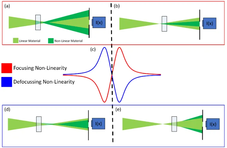
Chapter 4 discusses the physical properties of SA. This begins with a look at the linear character-istics including scattering, refractive index, and polarisation. These include small experiments to characterise these properties in samples fabricated in the methods outlined in Chapter 2. Following this the nonlinear optical properties are discussed and experimentally determined for SA. The main result being an optothermal nonlinear refractive index, determined through z-scan measurement. This property underpins all the major results of the thesis and is the mechanism by which scattering properties are altered and the NL-TM formed.

Chapter 5 begins the experimental exploration of nonlinear light scattering manipulation by demonstrating the manipulation of the far field intensity of weakly scattered light in SA. This is achieved using a parallel pump-probe PP optical setup to simultaneously locally deposit heat and record scattered intensity, which will become a familiar feature of experimental work in this project. After demonstrating this manipulation experimentally, results are backed up through simulation. Here we use a split-step beam propagation method (BPM). Through this the change in refractive index due to optothermal nonlinearity can be understood.

Chapter 6 looks at a further particular application of nonlinear perturbation, the optical memory effect. Normally this is seen through small amounts of tilting or shifting of a coherent light source in relation to a material. Here we show that the nonlinear perturbation of SA through further PP experiments is an additional method by which to achieve this effect. This is termed the "nonlinear optical memory effect" (NL-OMEM).

(17)

1.3. Structure of the thesis

Finally, chapter 8 is the conclusion. Here the main points are summerised, discussing how this work has built upon previous studies in the field. The potential for development of the work presented here is also discussed.

(18)

C

hapter

2

Background and Theory

This chapter discusses various formalisms of light scattering as it pertains to the work in this project. It begins with a broad look at various light transport regimes from ballistic to diffusive, as well as the intermediate mesoscopic scattering regime. We discuss light scattering in the context of the microscopic wave equation, which leads to the ideas of reciprocity and information preservation as light transports through a medium.

Next, we will discuss the field of "wavefront shaping," an iterative method of wavefront optimisa-tion that was developed as a means of tailoring the properties of a scattered wavefront in time, space, polarisation, or even wavelength. However, this method still treats a scattering material as a form of "black box," optimising an input iteratively until a level of desired output is found. Following this, the "Transmission Matrix" (TM) formalism will be discussed both theoretically and how it is implemented experimentally. The TM provides a complete description in how light scatters through a given material such that light scattering can be controlled deterministically

2.1 Light Scattering Regimes

Photons are rarely observed directly from their source. When viewing everyday objects such as a house or car, we only see them as a result of scattering or diffuse reflections from their surface. However, there are much richer descriptions behind these phenomena than light simply being scattered or directly observed. A whole spectrum of light transport mechanics exists between the two, with a vast array of mathematical and scientific theories describing them.

Light travel with no scattering events is known asBallistic Transport. Here the path of light is very well defined and can be predicted accurately with little computational effort. The vast majority of common optical elements deal with manipulating light in this regime. Lenses have a well defined focal length and focus light down to readily determinable spot sizes. We can easily control polarisation; mirrors reflect light directly and predictably. How these optical elements modify the optical wavefront can be described mathematically by theirTransmission Matrix(TM). These typically small matrices (2x2 for ballistic light transport) mathematically link input and output wavefronts and can also be combined through matrix multiplication to describe the effect of a whole array of optical elements in tandem.

(19)

2.2. Light Scattering as an Optical Tool

as an optical tool. With the correct choice of diffusion constants, it is possible to use the diffusive regime as a tool for invisibility cloaking [18].

Another approach to multiple scattering is one which retains the wave-like nature of light and is known as mesoscopic scattering physics. Under this formalism, and as will be discussed in detail, it has recently become possible to determine the TM of strongly scattering elements, a matrix of vastly more elements and the tensorial link between input and output wavefronts, through a set of techniques known as wavefront shaping [1]. These techniques have allowed for the creation of a wide variety of optical tools, such as perfect mirrors [19],high resolution spectral filters [20], or polarization sensors [21]; from simple scattering elements. It is the mesoscopic treatment of the multiple scattering problems that is of appropriate use in this project.

In between the two, and also of significant interest for this project is theweaklyor single scattering regime. Here light undergoes either one or few scattering events travelling through a material of a given length. Typical examples include the atmosphere or certain colloids. The shape, size, and distribution of the scatters determine the angular distribution of light intensity scattered at a given wavelength, known as thescattering phase function.

While here three distinct scattering regimes have been described here, light transport exists on a continuous spectrum, and sometimes it can be challenging to determine the correct regime and corresponding descriptive mathematics which are best suited for a given scenario. As a general rule of thumb, scattering intensity can be used to determine the best regime to use. At a given depth,τ, known as the optical depth, the intensity of a beam passing through a scattering material is reduced to exp(−τ)of its original level. If τ<0.1 then single scattering is the dominant process. For 0.1<τ<0.3 there will be more than one, but still few scattering events. Whenτ>0.3, multiple scattering processes dominate [22].

2.2 Light Scattering as an Optical Tool

The propagation of light in any medium, regardless of the scattering type, can be described by the (microscopic) wave equation [4]:

∇2ψ(r,t) = n

2₍_r₎

c2

∂2ψ(r,t)

∂t2 (2.1)

Whereψ(r,t)is the complex electric field of the light beam. When calculating transport through clear media, n(r), the refractive index, is a constant. Scattering is caused by variations in n(r), typically through the existence of small particles, or variations in material density.

One of the most commonly used and most well-studied instances of light scattering in photonics is the speckle pattern. The interference of light forms speckle patterns as it travels through multiple scattering media. Consider a laser beam impinging on such material. Initially all the photons are in phase, however, after passing through the media, they will have undergone different scattering events and as a result, taken differing paths. At the output plane, photons at a given point will have phase determined by the total optical path length they took. How these photons with random phases constructively and destructively interfere determines the brightness at that point.

(20)

2.3. Wavefront Shaping

These concepts, the randomisation of phase by scattering, no loss of information, and reciprocity, lead to the ideas of wavefront shaping, where input light is manipulated iteratively to illicit a desired output response, and the TM formalism which can entirely and uniquely describe how light scatters through a given material.

2.3 Wavefront Shaping

We consider now a picture of light undergoing multiple scattering in 2.2. As information about the wavefront has merely been scrambled in a set fashion, if the phase shift of scattered photons could be pre-compensated for, photons impinging at a point on the output plane would could all have the same phase, constructively interfere, and create an extremely bright speckle point.

Control over a light source in the optical regime for this compensation and other manipulations has been revolutionised by the advent of the Spatial Light Modulator (spatial light modulator (SLM)), allowing for a pixel by pixel manipulation in the wavefront of light. Manipulations such as this are known as wavefront shaping. We first describe the operation of the SLM before going on to discuss wavefront shaping.

2.3.1 The spatial light modulator

The SLM functions like a liquid crystal display (LCD). Its major components can be seen in 2.1. A CMOS circuit at the rear of the device applies a voltage between the pixel and transparent electrodes. To each of the electrode’s pixels, we can apply different voltages. In between the electrodes is a liquid crystal layer. This layer is composed of uniaxial organic molecules that align themselves to an applied electric field. Finally, the system is encased in glass, typically with an anti-reflection coating. For the SLM used in these experiments, this is at 532nm.

When a voltage is applied to a given pixel, the molecules in front of that pixel begin to rotate. The voltage can be increased to the point that the molecules have fully aligned their long axis with the electric field. As these pixels are birefringent, the refractive index and therefore phase delay at a given pixel is dependent on the applied voltage. A 0 to 2πphase delay is possible from the two passes the light makes through the system. To fully take advantage of the phase delay capability, the polarisation of the incoming beam but be aligned correctly. For the SLM used here, as with most SLMs, this a vertical alignment. When polarised in this way, this is known as operating the SLM in "phase-only mode." With most SLMs, there are additional "Amplitude" and "Amplitude and Phase" modes, by using different input polarisations. While we could, in theory, use these modes for these experiments, they both function by the removal of light from the optical system. In order to perform experiments as quickly as possible, with the lowest exposure time in the Charge-coupled device (CCD) camera, we run the system in phase only mode.

The SLM is attached to a PC which treats it as a 2nd monitor. We display greyscale images on the 2nd monitor, with the greyscale value (0-255) of each pixel determining the voltage which is applied by the SLM at that pixel. Therefore, the greyscale value determines the phase delay imparted to that area of the wavefront. Typically, the full range of greyscale values relates to a 0 to 2πphase delay. However, this relationship is rarely linear. We compensate for this by a look up table (LUT). The LUT is provided by the SLM manufacturer, which compensates the system into a linear relationship between greyscale value and phase.

(21)

[image:21.595.97.514.110.446.2]

Figure 2.1: Schematic of the spatial light modulator. Individual pixels can be addressed with a voltage, changing the refractive index of the liquid crystal in front of the pixel. This allows us to pattern the phase of a reflected wavfront, allowing for wavefront shaping

the 1st diffracted order. This technique removes phase imperfection induced by the periodicity of the pixels in the device. However, coupling to the 1st diffracted order is not 100% effective, and some light will continue to propagate in other orders

2.3.2 Wavefront shaping for light focussing

Vellekoop and Mosk did the fundamental work in wavefront shaping in the optical regime [2]. In this work, initially, a laser source first goes through polarisation optics. For the SLM to modulate only the phase of the wavefront and not the amplitude, the polarisation must be aligned correctly. The correct orientation depends on the device.

(22)

Figure 2.2: a) Light scattering through media that has not undergone wavefront shaping. Combina-tions of destructive and constructive interference create a speckle pattern on the output plan. In this case, destructive interference has occurred. b) Light scattering through a media that has undergone a wavefront shaping optimisation. Here the resulting constructive interference has created a point of high intensity at a chosen point in the output plane.

Figure 2.3: Various phase control algorithms used for wavefront shaping experiments. a) Sequential Algorithm. b) Continuous Sequential Algorithm. c) Partitioning Algorithm

and for solid samples (like the SA used for this project) hours. The longer a sample remains in the same state, the more iterations of an algorithm can be performed. Different algorithms also perform better/worse depending on the signal to noise ratio (SNR)s as the phase is modulated. Apart from the choice of algorithm, the other variable for optimisation is the resolution of the modulation. This is controlled by "grouping" pixels on the SLM together into segments, N. The more segments that are used the higher FOM that is reached, however the slower the algorithms become to iterate. If the goal of the optimisation is to generate a bright focus point, It has been shown that the intensity of the generated focus is directly proportional to the number of segments that are modulated.

(23)

One of the advantages of this algorithm is that it is guaranteed to reach a "global maximum," i.e. the best possible solution, in a single iteration. Ensuring the finding of a global maximum is something that must be considered in all searching algorithms. In algorithms that have continual improvement in FOM, solutions may be found that are not the best possible solution to the problem. This is because deviation from any maximum FOM is considered a worse solution, regardless if an even higher FOM exists elsewhere. In genetic algorithms for example, a randomness added to each phase profile during iteration can mitigate this problem.

The disadvantage of this algorithm is two-fold. Firstly, altering one segment at a time is a slow process and therefore is not appropriate for samples with short persistence times. Secondly, since only one segment is altered at a time, the variation in intensity during modulation is low, i.e a low SNR. In both cases adjustment on the number of modulated segments may be needed.

The algorithm used in b) is similar to the first, and is known as thecontinuous sequential algorithm. The only difference here is that after each segment is modulated, it is kept at its optimised value. When trying to generate a focus point, in this algorithm, the FOM target intensity improves with each optimised segment. This mean that SNR improves over time.

Algorithm c) is known as thepartitioning algorithm, this algorithm aims to overcome the previous weaknesses of SNR in the other two algorithm. Here a random 50% of segments are modulated together. This results in a larger change in FOM during modulation, improving SNR. This algorithm runs indefinitely, which a different random 50% selected in each instance.

When a suitable choice of an algorithm is made, the phase is then optimised. After which the modulated beam is focused through the scattering sample between two microscope objectives. The objectives reduce the number of transmission channels the light passes through, making it easier to achieve phase optimisation. The sample is also placed between two crossed polarisers, ensuring that only scattered photons are imaged. Vellekoop and Mosk achieved a focus with an intensity that was 1000 times brighter than the original speckle pattern [2].

2.3.3 Further experimental realisations of wavefront shaping

Rather than using a scattering material to focus light through, we can also focus inside materials. Vellekoop et al. followed this work up by using a fluorescent probe as a "guide star" [25]. The maximum level of optimisation, η, that is achieved in this way is related to the total number of controlled incident modes, or the number of independent modes of control on the SLM, N by the relation η = Nπ/4. Enhancement levels of up to 1800 times have been reported [2]. Such levels cannot always be reached depending on various experimental factors such as SNR and the effectiveness of enhancement detection. Overall such techniques have led to scattering materials have enhanced the ability of lenses to operate beyond the diffraction limit [26].

A natural extension to focusing light through one region of multiple scattering material is to transmit light through to multiple regions. As discussed earlier in the chapter, this due to the existence of "open channels," which are present in all scattering materials. Wave-front shaping provided the first experimental observation of these channels [27]. When producing an optimised focus, in this case, a 700x enhancement, it was found that the transmitted intensity in the surrounding region also increased by 40%, this effect was also confirmed later through numerical simulations [28].

(24)

2.4. The Transmission Matrix Formalism for Scattering Materials

closely linked. Tuning the phase of multiple spatial components allows us to control the relative phase and amplitude of frequency components, allowing for transmitted speckle patterns to interfere constructively at a given time [32] [33] [34].

Examples of this include work by Aulbach et al., who demonstrated spatial wavefront shaping of a pulsed wavefront, optimising in both space in time. [32]. This ability is enhanced in both space and time with the inclusion of nonlinear effects [35], such as two-photon fluorescence microscopy [36].

Finally, the method of wavefront shaping extends beyond the goal of controlling light in its amplitude and phase. As long as a variable is measurable, an optimisation is possible. For example scattering materials have been turned into polarization sensors [37] [38], and wavelength sensors [20] [39] [21].

2.3.4 Dynamic wavefront shaping

The wide range of examples given here on the uses of wavefront shaping all use static media and will be the only type of media used in this PhD, however, a summary of dynamic wavefront shaping will be given here for completeness. If a media is dynamic and changes over time, the wavefront shaping process is continuously optimising against a changing set of conditions. The faster a material changes, the lower the optimisation at a given optimisation speed.

In this way material is characterised by its speckle de-correlation time, known as the persistence time,Tp. The maximum level of enhancement in this case, and by using a phase modulated SLM, is

given byηmax≈πTm/4Tp[2]. WhereTmis the time for a single measurement.Tmcan be reduced

drastically by wavefront shaping not with an SLM, but with a digital micromirror device (DMD), which operate on the order of 20Khz, orders of magnitudes quicker than SLM based measurements on the order of [40]. By using these faster classes of devices, focusing through dynamic media with various persistence times have been achieved [7]. However these faster devices do come with a cost, a binary nature of optimisation has a lower potential of final enhancement of an output. Intensity only optimisation like this has a maximum enhancement ofηmax ≈Tm/4πTp[41].

Overall there is progress yet to be made towards one of the "holy grails" of wavefront shaping, and that is to achieve microscopic resolution inside strongly scattering media [42]. There are no limitations on a theoretical basis that prevent this goal from being reached. However, there are experimental bottlenecks, the main one being the PC which processes the feedback algorithm. Though promising solutions are beginning to be to this can be found to this, such as custom hardware to process the algorithm specifically [43].

2.4 The Transmission Matrix Formalism for Scattering Materials

Rather than treating a scattering media as a "black box" where the input is manipulated iteratively to achieve the desired output, it would be more desirable to have a formalism that connects the incoming and outgoing flux in the system, and at the same time providing statistical information that can be used to determine material characteristics. The TM formalism provides a means to do that.

(25)

Figure 2.4: Waveguide modes travelling through a scattering medium, with boundaries in the transverse direction.

the "optical memory effect (OMEM)," the subject of an investigation in a later chapter. The finite number of options present for transport are known as "channels."

The transmission matrix can also be written directly, in terms of the input and output fields its links together:

Eout=tEin. (2.2)

WhereEoutis the electric field at the output plane of scattering material,Einis the electric field at the input plane, andtis the TM.

With this notation, if we were to determine the output at themthmode as a result of n input modes, it would be determined by the following relation:

Eoutm =

∑

n

tmnEinn. (2.3)

Where tmn is a single element of the TM. This formalism is not just limited to applications

involving the amplitude of electric fields. The TM generically links input and output, and as such can be used in the transformation of other properties of waves, such as wavelength, polarisation, and time.

The TM contains within it a wealth of statistical and mathematical information on the scattering properties of a medium. In order to understand this, the formalism will be now derived from first principles, following which additional statistical and mathematical properties will be explored. For reference, this formalism is described in further detail out with the scope of this project by Rotten and Gigan, in their review titledLight Fields in Complex Media, Mesoscopic Scattering meets Wavefront

Control[44].

As a model for this, consider a slab of scattering material of length L and width D, contained inside a perfect waveguide, figure 2.4, where light enters the left-hand side travelling in the +z direction and can only exit in the +z or -z direction. In the uniform regions, far from the scattering medium, light at each side of the waveguide can be decomposed into waveguide modes in the transverse direction.

The waveguide modes are given by:

χn(y) =

√

2/Dsin(nπy/D), (2.4)

(26)

ψω(x) =

N

∑

n=1

c+_α_,nχn(y)e ikx

nx

p kx

n

+c−_α_,nχn(y)e −ikx nx p kx n (2.5)

Here, all possible basis states were summed over N = ωD/cπ, for which the propagation constant kxn =

p

ω2/c2−(nπ/D)2 is real. Imaginary propagation constants result in evanescent modes with asymptotic decay. c±are complex coefficients which describe the right-moving (+) and left-moving (-) waves respectively. pkx

nis a normalisation constant which ensures each mode has

the same flux in the longitudinal (y) direction.

With this representation, the scattering matrix,S, is defined as a complex matrix which connects the incoming expansion coefficients with the outgoing ones, in other words connecting the incoming and outgoing modes of the waveguide.

cout=Scin cin=

c+_l c−r

cout=

c−_l c+r

(2.6)

Forcin,c+_l represents flux from the left side of the waveguide travelling in the +z direction and

c−r represents flux from the right hand side travelling in the -z direction. Conversely forcout,c−_l

represents flux from the left side of the waveguide travelling in the -z direction andc+r represents

flux from the right hand side travelling in the +z direction. In other words, the scattering matrix considers both reflection and transmission from a media with flux impinging on the right and left side of the material.

For each side of the material, the amount of light exiting the left-hand side of the waveguide will be the summation of the flux that has transmitted from the right travelling to the left, and the flux travelling from the left, which is reflected. The converse is true for the right-hand side of the waveguide. We describe this by the following relations

c−_l =r c+_l +t0c−r c+r =t c+l +r 0

c−r (2.7)

Wheretis known as the transmission matrix (TM) and represents the transformation of light modes inputted from the left side of the waveguide and outputted to the right. Furthermore, t0 represents the transformation of light modes inputted from the right side of the waveguide and outputted to the left. The symbolsrandr0 similarly represent reflection.

As applied to the field of wavefront shaping, we are only interested in light, which after being modulated by an SLM, transmits from one side of the material to the other. Considering equations 2.7 in light of this, we reduce the above relations without loss of generality:

c+r =t c+l (2.8)

Therefore for a complete description of this scattering system, only t, the TM, needs to be considered.

Transmission Eigenchannels

While the TM is certainly a potent tool, which we utilise later this chapter and in chapter 7, it is at first glance almosttooinformation rich. Comparing two TMs from two completely different systems side by side, one would be hard-pressed to link a matrix to a particular system.

(27)

Beginning again from the scattering matrix, which from the above relations, can be described by a 2x2 block matrix.

S=

r t0 t r0

(2.9)

Where † is the complex conjugate transpose of a given matrix. Next, assuming the waveguide system has no scattering or absorption losses.

∑

n

|cin,n|2=|cin|2=|cout|2=

∑

n

|cout,n|2 (2.10)

where |c_in|2₌_c†

incin, |cout|2=c†outcout (2.11)

∴c†_incin−c†outcout=0 (2.12)

By introducing the definition of the scattering matrix|cout|=Scin:

c†_incin−S†c†inScin

∴ c†incin(S†S−I) =0

(2.13)

WhereIis the 2x2 identity matrix. For the relation in equation 2.13 to be true,

S†S=I (2.14)

This means that the scattering matrix,S, is a unitary matrix, meaningSS†=Iis also true. Unitary scattering matrices indicate that flux is conserved in a system. Along with the above conservation condition, we can re-expand the scattering matrix into its constituent block matrices to come to a further set of conditions that the transmission and reflection matrices must satisfy.

r† t0† t† r0†

r t0 t r0

= 1 0 0 1 (2.15)

∴ r†r+t†t=1 (2.16)

t0†t0+r0†r0 =1 (2.17) Considering again for our purposes only light which originates from one side of the waveguide (non-primed), the Hermitian Matricestt†,t†t,rr†,r†rcan be used to describe scattering characteristics. For example, since we know that the diagonal of Hermitian Matrices are real and from the invariance property of the trace, that the total transmissionTand reflectionRcan be written asTr(t†t) =_∑_nτn

and Tr(r†r) = _∑_nρn respectively. Hereτn andρn are defined as the transmission and reflection

eigenvalues of the scattering system.

Now considering the TM,t, specifically, the number of input and output channels are given by the surface area of the input and output flux plane. In the case of our artificial waveguide, this surface area may be identical by construction; however, in reality, this is incredibly unlikely. Even if the areas were identical in the range ofmm2_{, on smaller scales, the surface roughness of each plane}

would be different, and as a result a different number of channel for input and output. Therefore we must generalise, and treattas a rectangular matrix of MxNelements as described previously. In this case, it is not possible to determine the eigenvalues fort, as eigenvalues cannot be defined for a rectangular matrix.

(28)

[image:28.595.134.475.116.329.2]

Figure 2.5: Bobby Fleming demonstrating the principle of SVD as it pertains to 2D matrices. In this case image form. Left: The raw image data containing 4032 unique row vectors. Right: Reconstructed images using SVD, each one using a linear combination of a various number of independent vectors.

t=UΣV† (2.18)

WhereΣis a diagonal matrix containing the singular valuesσi.U,V†are also unitary and the

coloumns of which are known as the output and input singular vectors oftrespectively. Due to the diagonal nature ofΣ, we can also equate equation 2.18 to the summation of the outer products of the matrix multiplication:

t=UΣV†=

∑

i

σiui◦vi (2.19)

With the diagonal values ofΣ,σi arranges from highest to lowest by construction, the element

σiui◦vion the right of 2.19 becomes less significant as the summation progresses. In other words,

the matrixtcan be essentially recreated by using just the few first singular vectors and values of U,Σ, andV†. The matrices from these first few values contain the dominating characteristics of the matrixt.

The SVD, in essence, tries to reduce a rank K to a rank R matrix where the rank of a matrix is the maximum number of linearly independent columns or rows. The SVD takes a list of R unique vectors and approximates them as a linear combination of K linearly independent vectors.

As an illustration of this consider figure 2.5. On the left of the figure is a raw image. On the other side are reconstructed images using SVD. In the case N=1, this is an image reconstruction using just one vector with the single biggest contribution to the full data. Each row of the image is the same, just different "brightness." N=2 uses a linear combination of two different unique vectors and so forth. One can see that by using the ten most dominant of the 4032 total vectors (the number of rows in the raw image), we can make an excellent approximation of the image. At N=50, the approximation is near indistinguishable from the image.

(29)

it can be said that the SVD characterises the significance of various input channels on the final output flux, in other words,σiis related to the transmission eigenvalues,τi, mentioned previously.

Equation 2.19 is used to determine the relationship between t,tt†, and t†t. Starting from the definition of the SVD:

t=UΣV†t†= (UΣV†)†=VΣ†U† ∴tt†=UΣV†VΣ†U. (2.20) Remembering thatVis unitary(V†V=I)andΣis a real diagonal matrix(ΣΣ†=|Σ|2₎_:

tt†=U|Σ2|U†. (2.21)

Conversely:

t†t=V|Σ2|V†. (2.22) As we earlier defined the transmission eigenvalues of t†t as τ we can say that the non-zero singular valuesσioftare the square-roots of the non-zero eigenvalues oftt†,tt†i.e.

tt†=UτU† t†t=VτV† (2.23) Here the diagonal ofτare the transmission eigenvalues in order of magnitude along its diagonal. Importantly this result demonstrates the reciprocity in light scattering statistics (in the absence of effects such as absorption and gain etc). From 2.23 we see that tt† and t†t contain the same eigenvalues. From this and the relations in 2.15 ,t0†_t0_,_t0_t0†_{, 1}₋_r†_r_{, 1}₋_rr†_{, 1}₋_r0†_r0_{, 1}₋_r0_r0†_{also have}

the same eigenvalues. This means that for a particular transmission channel from input modemi to

output modenj, the amplitude of transmission and reflection is the same from input modenj to

output modemi[45] [46].

2.4.1 Transmission Channels and the distribution of transmission eigenvalues

The SVD is a powerful tool in the analysis of the scattering matrix and by extension the TM. As mentioned previously, the SVD allows us to identify trends and the strength of trends within each dimension of a 2D matrix, and it is this that gives rise to the description of transmission channels. This is not the only use of such a technique. The SVD has also been used to maximise energy transport in scattering media [47], and identify individual absorbing targets as well as the wavefront required to focus on said targets [48]. However, this use of SVD for the determination of transmission eigenvalues and their distribution, as well as the determination of other associated statistics of the TM.

Rather than going through the difficult (if not impossible as will be discussed shortly) process of measuring a complete TM, random matrix theory (RMT) can be used to understand the statistical properties of a TM purely. The underlying assumption here is that a chaotic scattering system functions no differently than a set of random matrices that have suitable chosen properties. One such method is known as the "Mexico approach", which was the first method used to determine the distribution of transmission eigenvalues theoretically [49] [50] [51]. In this approach, the scattering matrix is replaced by random complex numbers. These random elements, however, must result in a matrix whose properties are the same as the scattering matrix. The random transmission matrix (RTM) must be unitary, as well as symmetric in the case of time reversal symmetry. Time reversal symmetry, as mentioned previously, is relevant in systems where effects such as absorption and gain are not present, as is the most relevant condition for this thesis.

(30)

Figure 2.6: Binomal distribution of eigenvalues in a fully measured TM.

P(τ) = 1

πpτ(1−τ)

(2.24)

From a physical standpoint, we understand the origin of a bi-modal distribution by considering a scattering system classically, where we treat the photons as particles only, and we neglect wave-like effects such as interference. A photon which enters the left-hand side of the bounded scattering waveguide system will give one of two outcomes. It will either be scattered and reflected out the left-hand side, resulting in a transmission eigenvalue for that channel ofτ=0, or transmitted out the right-hand side resulting in a transmission eigenvalue for that channel ofτ=1. Obviously, we cannot neglect interference effects entirely, but it does qualitatively explain the bi-modal distribution, as the probability of a channel having a given eigenvalue diminishes away from the classically allowed values.

One other aspect of this distribution that is of experimental importance is the peak towards τ=1, suggesting that there are a not insignificant number of transmission channels in which light transmission is near unitary. These are known as "open channels." [54] [55].

(31)

capturing information in the required resolution, not all photon exit angles will be captured by an imaging lens. Also, these experiments are performed in open slab geometry in contrast to our theoretical assumptions, resulting in a further loss of information. The experimental approach is still valid, however, in fact as will be shown later, measurement of such a small subsection of the total possible channels in no way impacts the vast array of powerful optical effects possible. However, it does raise questions as to the validity of the bimodal distribution of transmission eigenvalues in the transmission regime.

The experimental measurement process of the TM does not determinetin its entirety, rather it measures a random subset of the matrix, modified by the fact that light must travel from the exit of the system to a detector through air. This is termed ˜tsuch that the input and output fields are now linked by modified relations:

˜

Eout=˜tE˜in (2.25)

As a result of this subset measurement, the previous assertions on TM statistics are now invalid. The measurement is now that of a completely random matrix. How might this affect the statistics of the SVD? In this case, the singular valuesσioft, related to the transmission eigenvaluesτbyτi =σ_i2, follow the Marcenko-Pasture law [56]. The law describes, that for a random matrix of NxM elements, whereM>N, the distribution of the normalised singular values (normalisation in the case of TMs is by the average transmission), depends only on the ratioγ=M/N.

Figure 2.7 show examples of such probability distributions. One particular example of note is the case ofγ=1, where the distribution of singular values are tightly bounded between the interval

[0, 2]. These values are allowed to be greater than one by the normalisation to the mean intensity. However these values are not completely bounded, and there is an exponentially decreasing chance of finding singular values outside of this domain.

These rouge values are essential in the description of several scattering processes; for example, they can indicate the realisation of selective focusing on gold nanoparticle targets [57].

The probability distribution of transmission eigenvalues is not the only way to determine information on the scattering system. Plotting the distribution of values themselves also yields interesting phenomena. According to work by Dorokhov, the distribution of eigenvalues in RMT is given by the following relation:

τ2=sech2(Γ/2) (2.26)

WhereΓ is a random real and positive diagonal matrix. As mentioned previously, the total transmission is linked to the transmission eigenvalues byTtot =hτ2i. To adhere to this normalisation, maximum value of the diagonal elements are set toηmax, which is related to the total transmission

(which can be set arbitrarily between 0 and 1 for the purposes of this discussion) by:

Rηmax

0 sech2(η/2)dη

ηmax

=Ttot (2.27)

The interesting consequence to this relation is that no matter the value of Ttot, there exists

(32)

Figure 2.7: Normalised distribution of singular values , ˜σas a function of the ratio,γ, between the number of input and output modes, M and N.

2.4.2 Measuring the TM

There is a range of methods by which to determine the complex TM. In the vast majority of published experimental work, and as is the case for this thesis, the primary concern is with the determination of the phase portion of this matrix. The most common way to address the different modes of scattering materials is via an SLM.

Popoff et al. performed the first measurement of the optical TM [58] [1]. (Note: All references to measuring the optical TM refer to a partial measurement, as we do not access all input modes with the SLM, only a random basis subset.). Here, the complex optical field is accessed through the "full field interferometry method" [59].

Consider the intensity at a given output mode,Im, which is the result of interference between a

given mode and the reference field. This is also given by the square of the amplitude of the electric field, termed Eoutm . In this wayEoutm has two components:

Eoutm =sm+E_mout₍_controlled₎. (2.28)

Wheresm is the complex reference field and Eout_m₍_controlled₎ is the portion of the field in which

contains the controlled input modes. Using the definition of the TM in equation 2.3:

E_mout₍_controlled₎= N

∑

n

(33)

[image:33.595.197.436.136.342.2]

Figure 2.8: Examples of the Hadamard Basis. White represents areas of amplitude +1, and areas of black -1.

The intensity of a given output mode can now be given by:

Im =|Emout|2=|sm+ N

∑

n

tmnEnin|2. (2.30)

From equation 2.30, we must isolate the component of the TM,tmn. In order to do so, we modulate

the relative phase of the input modes. There are four of these shifts, given byα=0,π/2,π, 3π/2. Doing so transforms the equation to:

Iα

m=|Eoutm |2=|sm+ N

∑

n

eiα_t

mnEinn|2. (2.31)

Expanding:

Iα

m=|sm|2+| N

∑

n

eiα_t

mnEinn|2+2R(eiαsm N

∑

n

tmnEnin). (2.32)

By computingIm0,Imπ/2,Imπ,I3mπ/2,smtmncan be determined by:

smtmn =

(I0

m−Imπ)

4 +i

(I3π/2

m −Imπ/2)

4 . (2.33)

Typically, and as is the case in the work by Popoff et al. the modulation of the amplitude of the input modes takes the form of the Hadamard basis. This+1/−1 basis is useful as SLM pixels can never be turned "off" (figure 2.8). The role of each mode is found by a unitary transform back into the SLM basis.

(34)

Figure 2.9: Example cosine modulation of a single mode as a function of shifting its relative phase. The amplitude and phase of this modulation form the amplitude and phase of a given element in the TM.

the input modes at different frequencies, then Fourier transformed the results to determine the individual elements of the TM [60].

Measurement is also not limited to purely optical responses. In work by T. Chaigne et al., the photoacoustic transmission matrix was measured [48]. While photoacoustics does not feature in this thesis, some of the measurement method relates to how we measure the TM in this work. Here input mode(s) of some basis are shifted in relative phase, generating a cosine intensity modulation, the amplitude and phase of which form a given element in the TM. This is shown in figure 2.9.

2.4.3 Using the TM

The TM, one part of the full scattering matrix, is a complete description of the transportation of light through a scattering material. Localising light to a given region is the equivalent of measuring a single row of the TM. Before discussing the various experimental application of the TM, we will now look at the detail behind this claim, discussing the TM based approached to localising light into one region.

First, remember that the relationship between the output modes, input modes, and the TM (Eout,

Ein, andTmn =T) is given by:

Eout =

   

Eout,1

Eout,2

... Eout,m

    =  

t11 t12 ... ... t1n

... ...

tm1 tm2 ... ... tmn

  m×n      

Ein,1

Ein,2

... ... Ein,n

     

=T Ein, m<n (2.34)

(35)

suggest that in order to determine a givenEin, the TM is inverted. However, this is not an effective

way to determine the necessary input. The cause lies within the singular values. In a measured TM, the low singular values refer to noise. When the TM is inverted the singular values are also inverted, meaning that the noise becomes the greatest contributing factor, with the previous strong "trends" that the singular values represent becoming greatly diminished [58] [61].

A more robust approach is by employing time reversal. In contrast to TM inversion, time reversal ensures that energy continues to travel through the high transmission channels [58]. As mentioned in regard to equation 2.1, light exhibits time-reversal symmetry. In a general time reversal experiment, an array of transducers record the temporal modulation of a wave, then re-emits that signal in reverse. This was first experimental realisation of this was in works by Fink et al [62] [63] [64]. Here they scattered ultrasonic waves through an acoustically scattering medium composed of steel rods immersed in water. An array of transducers recorded the signal, which was approximately 100 times longer in time than the initial emission. By re-emitting this signal from the transducers in reverse, a signal was formed on the other side that was highly localised in both space and time. In this way, the transducers have formed what is known as a time reversal mirror.

Moving to the optical regime with time reversal is challenging as is requires both interferometry measurements as well as the shaping of light pulses simultaneously in amplitude and phase. Several experimental works on the spatio-temporal control of waves, are making progress in this regard [32] [33] [36], with further theoretical methods proposed [65] [66] [67] [68] [69] [70].

However, in regards to the work represented here, there is no focusing of light in time, as the experiments will work solely with monochromatic light. The monochromatic equivalent of time reversal is known as phase conjugation. In phase conjugation, we measure the phase of a wavefront (which is time-invariant, i.e. no localisation in time), after which the wave is re-emitted back with a conjugate phase. This is explained also in figure 2.10.

We, therefore, in terms of the TM, we reverse the system using the complex conjugate transpose of the TM [1] [58]. By displaying the phase conjugate of a row of the TM on an SLM, light can be re-directed into a single region. Such an effect has been demonstrated experimentally extensively [60] [61]. In this way, the required input,Ein, needed to desired output which will be termedEouttarget

is:

Ein =T†·Eouttarget (2.35)

Additionally, this also explains the origin of the focusing operator discussed earlier, following from the definition of the TM [58]:

Eout =T†·Ein =T·T†·Eouttarget (2.36)

Therefore if the actual output,Eout matches the target output, Eout_target, then T·T†will be the identity matrix. Therefore, the focusing operator can be used as a tool to verify the effectiveness of the TM measurement

2.4.4 Experimental uses of the TM

Owing to the large number of degrees of freedom used in the measurement of a TM, in addition to the framework being flexible to various types of inputs and outputs depending experimental goals, the TM formalism can be employed in a variety of ways.

Linear and nonlinear optical properties of silica aerogel

LINEAR AND NONLINEAR OPTICAL PROPERTIES OF

SILICA AEROGEL

Adam Colin Fleming

A Thesis Submitted for the Degree of PhD

at the

University of St Andrews

2019

Full metadata for this item is available in

St Andrews Research Repository

at:

http://research-repository.st-andrews.ac.uk/

Please use this identifier to cite or link to this item:

http://hdl.handle.net/10023/18557

Linear and Nonlinear Optical Properties of

Silica Aerogel

Adam Colin Fleming

This thesis is submitted in partial fulfilment for the degree of

D

octor of

P

hilosophy

at the

U

niversity of

S

t

A

ndrews

School of Physics and Astronomy

University of St Andrews

KY16 9SS

https://synthopt.wp.st-andrews.ac.uk

Candidate’s declarations:

Supervisor’s declaration:

Permission for publication:

Underpinning Research Data or Digital Outputs

Candidate’s declaration

Permission for publication of underpinning research data or digital outputs

Acknowledgements

Funding

Digital Outputs access statement

Collaboration Statement

Publications and Awards

Publications Resulting from this Work

Awards

Conferences

Summer Schools Attended

Contents

C

hapter

1

Introduction

1.1

Control of light in scattering media

1.2

Silica aerogels

1.3

Structure of the thesis

C

hapter

2

Background and Theory

2.1

Light Scattering Regimes

2.2

Light Scattering as an Optical Tool

2.3

Wavefront Shaping

2.3.1

The spatial light modulator

2.3.2

Wavefront shaping for light focussing

2.3.3

Further experimental realisations of wavefront shaping

2.3.4

Dynamic wavefront shaping

2.4

The Transmission Matrix Formalism for Scattering Materials

∑