A Lattice Test for Additive Separability
A Lattice Test for Additive Separability
Matthew Polisson
∗February 12, 2018
Abstract: We derive necessary and sufficient conditions for a finite data set of price and demand observations to be consistent with an additively separable preference. We do so without imposing concavity on any of the subutility functions or convexity of the budget seta priori, thereby generalizing earlier results. Our simple and intuitivelattice test easily accommodates departures from rationality, or errors, which subsequently facilitates a rich empirical analysis. We apply our econometric techniques to the food consumption of a panel of British households. The primary empirical finding is that additive separability has considerable success in explaining the data.
Keywords: additive separability, consumer demand, lattice test, revealed preference
JEL Classification Numbers: C14, C60, D11, D12
∗ Affiliations: School of Economics and Finance, University of St Andrews, Castlecliffe, The Scores, St
1. Introduction
The separability of a consumer’s preference—across goods, time periods, states of the
world, and so on—is a frequently held assumption in economics. Separability is useful
be-cause it restricts the attention of both the agent and the econometrician to a single
commod-ity or commodcommod-ity group, and this simplification pays dividends in numerous theoretical and
empirical settings. One might therefore want to test for the separability of a consumer’s
pref-erence, i.e., to characterize the empirical content of separability in the form of its implied
restrictions on observable data, which are typically prices and demands. The question of
separability and its empirical implications has therefore spawned a long and rich literature.1
Suppose that we have access to a finite data set containing price and demand observations.
In this paper, we derive restrictions on this data set which are necessary and sufficient for it
to have arisen from the maximization of a separable preference of a particular form known
asadditivity, which is a type ofstrong separability. We do so in the nonparametric revealed
preference tradition of Afriat (1967), Diewert (1973), and Varian (1982), i.e., we do not
assume anything about the specific functional shape of the preference, only the primitive
essentials. Furthermore, unlike previous revealed preference work on additive separability
(see Varian (1983), Diewert and Parkan (1985), and Fleissig and Whitney (2007)), we do not
require convexity of the preference or of the budget seta priori. Instead we extend thelattice
approach (see Polisson, Quah, and Renou (2017)) to achievedomain reduction; crucially, the
lattice approach does not appeal to the techniques of convex optimization, which allows for
an easy extension to accommodate departures from full economic rationality, or errors, in
the form of cost inefficiencies (see, e.g., Afriat (1972, 1973) and Varian (1990)).
We implement our procedures on a panel of British consumers known as the Kantar
Worldpanel, previously used to study nutrition in Dubois, Griffith, and Nevo (2014), among
some other papers.2 The data set is a representative sample of British households observed
1 For surveys on functional structure and separability, see Blackorby, Primont, and Russell (1978) and
Deaton and Muellbauer (1980); for seminal references on separability, see Leontief (1947), Strotz (1957, 1959), Frisch (1959), Gorman (1959, 1968), Debreu (1960), Houthakker (1960), Pearce (1961), and Goldman and Uzawa (1964); for nonparametric tests of separability in the spirit of those which are developed and implemented in this paper, see Varian (1983), Diewert and Parkan (1985), Swofford and Whitney (1987, 1988), Fleissig and Whitney (2003, 2007, 2008), Echenique (2014), Quah (2014), and Cherchyeet al. (2015).
between 2005 and 2012. We focus our empirical analysis on 4 aggregate food groups—fruit,
vegetables, red meat, and poultry/fish—and we explore the relationships within two
sub-groups: {fruit, vegetables} and {red meat, poultry/fish}. The primary empirical finding is
that additive separability has considerable success in explaining consumption choices within
both subgroups; this success is more pronounced within the subgroup {fruit, vegetables}
than {red meat, poultry/fish}, suggesting greater substitutability/complementarity within
the latter subgroup, or equivalently, greater demand independence within the former.
This paper is a contribution to the econometric investigation of the empirical content of
separability, and in particular, additive separability. It has long been thought that additivity
is extremely empirically restrictive, and that while often a convenient simplifying assumption
to make, it is unsuitable for applied empirical work due to the restrictions it imposesa priori
on substitution terms, and hence own- and cross-price elasticities of demand.3 However,
in this paper we argue that additive separability, in the absence of auxiliary parametric
assumptions and in the presence of finite data, may not be as restrictive as it might at first
appear. The remainder of the paper is organized as follows. Section 2 defines separability,
and in particular additive separability, and underscores its central role in simplifying the
economic analysis of consumer behavior. Section 3 outlines the revealed preference approach
as a means of characterizing the empirical content of additive separability. Section 4 describes
the empirical implementation and results. Section 5 concludes.
2. Separability
Suppose that a consumer has a rational preference ordering < over a consumption set,
which we assume to be R`
+. Further suppose that these commodities can be divided into
two commodity groupsX and Y. The consumption set is then given byX×Y, with typical
element (x, y). It is well known that preferences are separable on X if (x, y) < (x0, y) for
some y ∈ Y implies (x, y0) < (x0, y0) for all y0 ∈ Y, i.e., the weak preference of x to x0 is
as well as a discussion of the costs and benefits of using household scanner data (rather than conventional household surveys) to study nutrition.
3Deaton (1974) concludes “the main argument of this paper is thatthe assumption of additive preferences
independent of the choice from Y. It is also known that if < has a utility representation,
then preferences are separable on X if and only if there exist some functions v :X →R and
f :R×Y → R, where f is increasing in its first argument, such that u(x, y) = f(v(x), y).
Assuming differentiability, notice that the marginal rates of substitution between any two
commodities in X are independent of the choice from Y. We could of course separate the
preference even further, and the strongest form of separability typically invoked is additive
across all commodities, i.e., if there are ` commodities, then u(x1, x2, . . . , x`) =
P`
i=1vi(xi),
where vi : R+ →R for all i = 1,2, . . . , `.4 Again assuming differentiability, it is easy to see
that the marginal rates of substitution between any two commodities are independent of the
amounts of any other commodities. The literature on functional separability and its role in
the economics of consumer behavior is comprehensively summarized by Blackorby, Primont,
and Russell (1978) and Deaton and Muellbauer (1980).
The separability of a consumer’s preference is often an assumption made out of
neces-sity, either explicitly or implicitly. Any empirical work in consumer demand and industrial
organization necessarily focuses on a subset of products, the justification for which
typi-cally involves invoking some type of separability argument. It is therefore well known that
substitution patterns across groups are restricted a priori, e.g., across goods
(consump-tion/leisure), time periods (today/tomorrow), and states of the world (good/bad). In fact,
it is not uncommon to assume even stronger forms of separability, e.g., quasilinear
util-ity (e.g., in consumer demand, industrial organization, and mechanism design), exponential
discounting, and expected utility. Many of the canonical models in economics appeal to
separability as a simplifying device, and it is therefore unsurprising that we might want to
test for the separability of a consumer’s preference.
3. Revealed Preference
In this paper, we suppose that we have access to a finite set of price and demand
observa-tions taken from an individual consumer. Our revealed preference analysis is in the spirit of
Afriat (1967), Diewert (1973), and Varian (1982), i.e., we adopt a completely nonparametric
4 Interestingly, Debreu (1960) shows that a necessary and sufficient condition for additive separability is
approach rather than assuming that preferences take a specific functional form, which can
then be applied at the level of the individual consumer.5 This approach is in contrast to
conventional econometric approaches, which typically adopt functional forms and restrict
observed and unobserved heterogeneity a priori.6
3.1 Afriat’s Theorem
Let{(pt, xt)}T
t=1 denote a finite set of observations drawn on an individual consumer. At
every observation t = 1,2, . . . , T, an econometrician has access to the consumption bundle
xt= (xt1, xt2, . . . , xt`)∈R`
+ and the corresponding price vector pt= (pt1, pt2, . . . , pt`)∈R `
++.
Definition 1. For any consumption bundles xt, xs, the bundle xt is directly revealed
pre-ferred to the bundle xs (xt<∗
0 xs) whenever pt·xs6pt·xt.
Definition2. For any consumption bundlesxt, xs, the bundlextis directly revealed strictly
preferred to the bundle xs (xt ∗
0 xs) whenever pt·xs < pt·xt.
Definition 3. For any consumption bundles xt, xs, the bundle xt is revealed preferred to
the bundle xs (xt <∗ xs) whenever pt·xi 6 pt·xt, pi ·xj 6 pi ·xi, . . . , pk·xl 6 pk·xk,
pl·xs 6pl·xl.
In words, we have established thatxt is directly revealed preferred toxs if xs was affordable
when xt was purchased, and that xt is directly revealed strictly preferred to xs if, not only
wasxs affordable whenxt was purchased, but also it coststrictly less. The transitive closure
of the direct revealed preference relation then implies thatxtcan be revealed preferred toxs
either directly or through a chain. These definitions lead naturally towards what has become
a central axiom in the revealed preference literature.
Definition4. The data set{(pt, xt)}Tt=1 obeys the Generalized Axiom of Revealed Preference
(GARP) so long as xt <∗ xs =⇒ xs∗0 xt.
In words, GARP asserts that whenever xt is revealed preferred to xs, either directly or through a chain, it cannot be the case that xs is directly revealed strictly preferred to xt.
5See Chambers and Echenique (2016) and Crawford and De Rock (2014) for summaries of the theoretical
and empirical revealed preference literatures, respectively.
An equivalent statement is that whenever
xt<∗0 xi, xi <∗0 xj, . . . , xk <0∗ xl, xl <∗0 xs, xs <∗0 xt,
none of the weak relations (<∗0) can be replaced with a strict relation (∗
0). Therefore,
GARP is essentially an intuitive no-cycling condition on the data, and it is straightforward
to show that such a condition is a necessary consequence of maximizing a well-behaved utility
function. We now consider the problem formally.
Definition 5. The data set {(pt, xt)}Tt=1 is rationalizable if there exists a utility function
u:R`
+→R, such that, at every observation t= 1,2, . . . , T,
u(xt)>u(x) for any x∈Bt ={x∈R`
+ :pt·x6pt·xt}.
A data set is therefore said to be rationalizable if there exists a utility function, such that,
at every observation, the consumption bundle that was chosen delivers weakly greater utility
than any other consumption bundle that was affordable. This definition is both natural and
standard, and we can relate this rationalizability concept to GARP via Afriat’s Theorem.
Theorem 1. The following statements are equivalent:
1. The data set{(pt, xt)}T
t=1 is rationalizable by a nonsatiated utility functionu:R`+ →R.
2. The data set {(pt, xt)}T
t=1 obeys GARP.
3. For the data set {(pt, xt)}T
t=1, at every observation t= 1,2, . . . , T, there exist numbers
ut∈
R and λt∈R++, such that
ut0 6ut+λtpt·(xt0 −xt) for all t, t0 = 1,2, . . . , T.
4. The data set {(pt, xt)}T
t=1 is rationalizable by a utility function u : R`+ → R, which is
increasing, concave, and continuous.
Proof. See Afriat (1967), Diewert (1973), and Varian (1982).
Some brief remarks on Afriat’s Theorem are in order. First, the theorem characterizes
the observable restrictions on a given data set are both necessary and sufficient for utility
maximization, these restrictions exhaust the empirical implications of such a procedure.
Second, the theorem provides two equivalent empirical tests for utility maximization in a
finite data setting: one involves checking GARP, and the other involves finding a feasible
solution to a set of linear inequalities, which have come to be known as the Afriat inequalities.
Both procedures are computationally efficient. Third, in a finite data setting, if a data set is
rationalizable by a nonsatiated utility function, it is also rationalizable by a utility function
that is increasing, concave, and continuous. An equivalent statement is that monotonicity,
concavity, and continuity of the utility function are, over and above nonsatiation, without
loss of generality in a classical finite data setting, i.e., they are untestable. Since these
properties are without loss of generality, they can be assumed without cost in this setting.7
3.2 Additive Separability
Testing for separability is typically thought to be a ‘hard’ problem, if not in concept
then in computation and application. Nonparametric tests of weak separability date back
to Varian (1983) and Diewert and Parkan (1985), in which each of the subutility functions
is assumed to be concave and the budget set is linear, i.e., the characterization is not
com-pletely general. This approach gives rise to a nonlinear (bilinear) test, which is known to be
computationally hard, although some practical advances have been made, e.g., see Swofford
and Whitney (1987, 1988), Fleissig and Whitney (2003, 2008), and Cherchye et al. (2015).
More recently, Quah (2014) establishes a testing procedure for weak separability that does
not require convexity of either the preference or budget set, and which is in principle
im-plementable on finite data sets that are not too large, while Echenique (2014) argues that
separability is, in general, a computationally hard problem.
Contrary to these somewhat negative results on the nonparametric testing of weak
sepa-rability, we argue thatadditive separability in its strongest but most common form is exactly
and efficiently testable. Varian (1983) and Diewert and Parkan (1985) were again the first to
establish necessary and sufficient conditions for additively separable rationalizability. The
7These stronger assumptions give rise straightforwardly to a set of necessary and sufficient conditions on
Varian (1983) characterization partitions the ` goods into two groups, but the result can
easily be generalized to some number of groups less than or equal to `.8 What is critical is
that each of the subutility functions is concave and the budget set is convex, which allows
for a first-order condition approach (appealing to the techniques of convex optimization)
that produces a straightforward linear test. Varian (1983) and Diewert and Parkan (1985)
therefore establish a joint test for additive separability and global concavity of each of the
subutility functions, where the maximization of this preference is subject to a classical
lin-ear budget constraint. Notice that concavity of the subutility functions implies diminishing
marginal utilities of consumption in every commodity, which is akin to assuming a smoothing
of consumption across commodities (e.g., consumer products, time periods, and states of the
world). Nothing about additive separability as it is defined requires concavity of the
subu-tility functions or any such smoothing, and so a violation of the Varian (1983) and Diewert
and Parkan (1985) tests is not necessarily a violation of additive separabilityas such.
In this paper, we develop and implement a test of additive separability that does not
require concavity of the subutility functions a priori, nor does it require a convex budget
set. In this sense, we provide a more general test than Varian (1983) and Diewert and
Parkan (1985). Our results hold when all goods are additively separable, i.e., when there is
a subutility function associated with each good defined over the consumption space for that
good. In this sense, we are less general than Varian (1983) and Diewert and Parkan (1985),
although this stronger notion of additive separability is common in many applied theoretical
and empirical settings. Since we do not require convexity of either the preference or budget
set, the procedure can be extended to account for departures from rationality, or errors, in
the form of cost inefficiencies (see, e.g., Afriat (1972, 1973), Varian (1990), Halevy, Persitz,
and Zrill (2016), and Polisson, Quah, and Renou (2017)); as will soon be made clear, the
notion of Afriat (1972, 1973) cost inefficiencies requires a rationalization over a (modified)
nonconvex budget set, even if the budget itself is convex. As a result, what emerges is a
simple, intuitive, and easily implementable nonparametric test of additive separability in its
most common form, which allows us to reconsider the question of the empirical plausibility
of additivity in the absence of any confounding functional form assumptions.
3.3 A Lattice Approach
Before developing our revealed preference procedure, it is worth exploring what
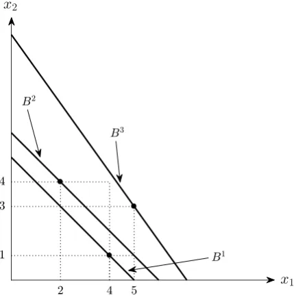
consti-tutes a violation of additive separability. Consider the example depicted in Figure 1. In this
simple example with two goods and three observations, the consumer purchased x1 = (4,1)
from B1, x2 = (2,4) from B2, and x3 = (5,3) from B3.9 Since none of the budget lines
intersect, it is immediate that these observations obey GARP and are therefore
rationaliz-able as having arisen from the maximization of a nonsatiated utility function. They arenot,
[image:10.595.199.414.266.487.2]however, rationalizable by additive separability, which is straightforward to demonstrate.
Figure 1: Violation of Additive Separability
At the first observation, it must be the case that v1(4) +v2(1) > v1(2) +v2(3), since
(2,3) was available when (4,1) was purchased; at the second observation, it must be the
case that v1(2) +v2(4)> v1(5) +v2(1) since (5,1) was available when (2,4) was purchased;
together these inequalities imply that v1(4) +v2(4) > v1(5) +v2(3), which contradicts the
third observation since (4,4) costs strictly less than (5,3) when (5,3) was chosen. What
this simple example illustrates is that an additive structure may give rise to further revealed
preference relations through a cancellation of terms,10 and this is precisely what we hope to
9 The prices have been suppressed since we do not require them for this example.
10In fact, Debreu (1960) shows that with only two goods, as in our example, if preferences are representable
systematically capture in our revealed preference approach.
The procedure we develop makes use of a revealed preference concept known as thelattice
method, which was first introduced by Polisson, Quah, and Renou (2017) in order to test a
broad class of models of decision making under risk and under uncertainty. The essence of
the approach is to achieve domain reduction, i.e., to convert (without loss) an infinite set of
revealed preference relations on the consumption space into afinite set of revealed preference
relations on the lattice. The latter, crucially, can be checked. In Polisson, Quah, and Renou
(2017), the lattice method allows for revealed preference tests of many different models of
decision making under risk and under uncertainty, and without requiring concavity of the
Bernoulli utility function a priori. In these settings, many utility representations take a
separable form, and so the problem in Polisson, Quah, and Renou (2017) has a functional
[image:11.595.197.414.338.563.2]structure similar to additive separability as described in this paper.
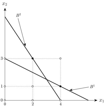
Figure 2: Rationalizability by Additive Separability
Before formalizing the main argument, we present another simple example in order to
develop intuition. Suppose that we have observed a consumer choosing the bundlex1 = (4,1)
at the prices p1 = (2,4), followed by the bundle x2 = (2,3) at the prices p2 = (3,2).
This situation is depicted in Figure 2. The data obey GARP since (4,1) was purchased
when (2,3) was unavailable, and vice versa, and therefore the data are rationalizable by
by additive separability, i.e., if there exist increasing and continuous subutility functions
v1 :R+ →R and v2 :R+ →R, such that
v1(4) +v2(1) >v1(x1) +v2(x2) for any (x1, x2)∈B1,
v1(2) +v2(3) >v1(x1) +v2(x2) for any (x1, x2)∈B2,
where B1 ={(x1, x2) ∈ R2+ : 2x1+ 4x2 6 12} and B2 = {(x1, x2)∈ R2+ : 3x1 + 2x2 6 12}.
Since we do not require that the subutility functionsv1 andv2are concave as in Varian (1983)
and Diewert and Parkan (1985), we cannot adopt a first-order condition approach when
deriving restrictions on this data set which are necessary and sufficient for rationalizability
by additive separability. Instead, we appeal to the lattice method.
Notice that for the first good, we have observed the consumption levels 2 and 4, and for
the second good, the consumption levels 1 and 3. At a minimum, the consumption set for
the first good must contain the elements in X1 = {0,2,4}, i.e., any observed consumption
levels plus zero, and similarly, the consumption set for the second good must contain the
elements in X2 = {0,1,3}. Consequently, the consumption set must contain, again at a
minimum, any elements in the finite lattice L = X1 × X2. It is certainly clear that as a
necessary condition for rationalizability by additive separability, there must exist sets of
real numbers {v¯1(0),v¯1(2),v¯1(4)} and {v¯2(0),v¯2(1),¯v2(3)}, with ¯v1(0) < v¯1(2) < ¯v1(4) and
¯
v2(0)<¯v2(1) <v¯2(3),11 such that
¯
v1(4) + ¯v2(1) >¯v1(x1) + ¯v2(x2) for any (x1, x2)∈B1∩ L,
¯
v1(2) + ¯v2(3) >¯v1(x1) + ¯v2(x2) for any (x1, x2)∈B2∩ L,
with the inequalities strict whenever (x1, x2) is in the interior of the budget set.12 This
simplifies to finding sets of real numbers satisfying ¯v1(4) + ¯v2(1)>v¯1(0) + ¯v2(3) and ¯v1(2) +
¯
v2(3)>v¯1(4) + ¯v2(0).13 It is clear that by letting ¯v1(0) = 0, ¯v1(2) = 2, ¯v1(4) = 4, ¯v2(0) = 0,
¯
v2(1) = 1, and ¯v2(3) = 3, we meet this requirement. If we were unable to find such numbers,
then we would reject that these data could have arisen from the maximization of an additively
11 This is due to monotonicity, i.e., the subutility functionsv
1:R+→Randv2:R+→Rare increasing.
12 This is again due to monotonicity.
13The simplification arises since elements of the lattice which are weaklydominated by the bundles chosen
separable preference. What we claim in this paper is that the above requirements are also
sufficient for rationalizability by additive separability.
We now address the problem formally. Below is the general notion of rationalizability by
additive separability to which we appeal throughout the remainder of the paper.
Definition 6. The data set {(pt, xt)}Tt=1 is rationalizable by additive separability if there
exist a collection of subutility functions {vi}`i=1, with vi :R+→R increasing and continuous
for all i= 1,2, . . . , `, such that, at every observation t= 1,2, . . . , T,
`
X
i=1
vi(xti)> `
X
i=1
vi(xi) for any x∈Bt ={x∈R`+ :p
t·x
6pt·xt}.
Notice thatall goods are additively separable in this formulation, i.e., the marginal rates
of substitution between any two goods are independent of the consumption of any other
goods. This strong form of separability is very common but thought to be highly restrictive.
Theorem 2. The following statements are equivalent:
(1) The data set {(pt, xt)}T
t=1 is rationalizable by additive separability.
(2) There exist numbersv¯i(xi)∈R for each xi ∈ Xi ={x∈R+ :x=xti for some t} ∪ {0}
for all i = 1,2, . . . , `, with v¯i(xi) > v¯i(yi) whenever xi > yi for any xi, yi ∈ Xi, such
that, at every observation t= 1,2, . . . , T,
`
X
i=1
¯
vi(xti)> `
X
i=1
¯
vi(xi) for any x∈Bt∩ L, (A1)
`
X
i=1
¯
vi(xti)> `
X
i=1
¯
vi(xi) for any x∈(Bt/∂Bt)∩ L, (A2)
where L=Q`
i=1Xi denotes a finite lattiace, and where ∂B
t={x∈
R`+ :pt·x=pt·xt}
denotes the boundary of Bt.14
Proof. The proof is given in the Appendix.
The necessity of statement (2) is a straightforward generalization of the principle outlined
in the earlier example. The intuition for the sufficiency of statement (2) is that conditional
14 Notice, therefore, that the interior ofBtis denoted byBt/∂Bt={x∈
R`+:p
on being able to find subutility functions restricted to the finite lattice, a set of increasing
and continuous subutility functions can extend these mappings to the entire space, i.e., we
can always ‘connect the dots’. A natural choice for each extension is a step function, which
is neither increasing nor continuous; the sufficiency argument shows that we can construct
piecewise linear extensions that are arbitrarily close to these steps.
While the lattice approach developed in this paper relates in concept to Polisson, Quah,
and Renou (2017), it differs on two important accounts: (1) here we construct some arbitrary
number`subutility functions, one foreveryconsumption good, each of which is required to be
increasing and continuous, rather that asingle Bernoulli utility function over state-contingent
consumption; and (2) our method of proof involves constructing subutility functions which
are piecewise linear, and this can be done explicitly, whereas Polisson, Quah, and Renou
(2017) must allow for sufficient flexibility in the curvature of the Bernoulli utility function in
order to accommodate a broad class of models of decision making under risk and uncertainty,
[image:14.595.197.414.383.603.2]and as a consequence, the proof by induction is significantly more complicated.
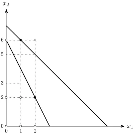
Figure 3: Violation of Concave Additive Separability
Returning to the example, we conclude that these data are, in fact, rationalizable by
additive separability. Furthermore, they are also rationalizable by concave additive
separa-bility (see Varian (1983) and Diewert and Parkan (1985)), i.e., the consumer’s choices are
had observed the consumer choosing the bundle x1 = (2,2) at prices p1 = (4,2), followed
by the bundle x2 = (1,6) at prices p2 = (2,2). The data clearly obey GARP, and it is
easy to show using the procedure described in this paper that they are also rationalizable
by additive separability. These data are not, however, rationalizable by concave additive
separability. Since (1,3) costs strictly less than (2,2) when (2,2) was chosen, it must be the
case that v1(2) +v2(2) > v1(1) +v2(3). By the concavity of subutility function v2, it must
also be the case that v2(6)−v2(3) 6 v2(5)−v2(2). Together these inequalities imply that
v1(2) +v2(5) > v1(1) +v2(6), which of course contradicts the optimality of (1,6). Intuitively,
since income increases and good 1 becomes relatively cheaper between observations 1 and 2,
a consumer who is smoothing consumption would never buy strictly less of good 1.
3.4 Departures from Rationality
So far the tests we have developed are forexact rationalizability by additive separability.
When a data set is not exactly rationalizable, it is imperative to establish some notion of the
‘distance’ from full rationalizability, or what we might callapproximate rationalizability. The
predominant convention in the revealed preference literature is to capture these departures
from rationality, or errors, in the form of cost inefficiencies. The stringency of a revealed
preference test can always be reduced by requiring a rationalization over the budget set
Bt(e) ={xt} ∪ {x∈
R`+ :pt·x6e pt·xt} for some e∈[0,1] for all t= 1,2, . . . , T. In other
words, a consumer maximizes subject to a degree of cost efficiency e. The largest value of e
which rationalizes a given data set is known as the critical cost efficiency index (CCEI) for
that data set. The basic idea is that the degree to which a consumer is cost inefficient is a
reflection of his departure from full economic rationality (see, e.g., Afriat (1972, 1973), Varian
(1990), Halevy, Persitz, and Zrill (2016), and Polisson, Quah, and Renou (2017)). Notice,
crucially, that the budget set Bt(e) is not convex.15 Since the lattice approach does not
require this, it can be applied straightforwardly to check for rationalizations on nonconvex
budget sets, and as in Polisson, Quah, and Renou (2017), this is one of its important features,
particularly with regard to empirical work.16
15 See Forges and Minelli (2009) for revealed preference tests on nonconvex budget sets. 16LetCt=Bt(e) ={x∈
R`+:x6xt} ∪ {x∈R`+:pt·x6e pt·xt}for somee∈[0,1] for allt= 1,2, . . . , T,
and apply Lemma 1 in Appendix A.2. Notice that{x∈R`+:x6xt}has replaced{xt} in the definition of
4. Implementation
4.1 Data
We apply our revealed preference procedures to a representative sample of British
con-sumers from the Kantar Worldpanel, which is a rolling panel of British households that
record (via a barcode scanner) all food purchases which enter the home. Data between 2005
and 2012 are aggregated to the household-year-month level, which is a convention in the
literature on the economics of nutrition, driven by practical aggregation considerations and
also by the need to treat a household’s food purchases as non-durable and non-strorable
across observations.17 We subsequently drop any household-year-months over which a given
household has not made a purchase for 7 or more consecutive days in order to exclude any
infrequencies. We then restrict our sample to a subsample of households that have been
observed for at least 50 year-months, and for each of these households, we randomly select
50 of these year-months. The final sample therefore contains 4,027 households, each of which
has been observed on 50 occasions.
We focus our empirical analysis on 4 aggregate food groups: fruit, vegetables, red meat,
and poultry/fish. It is standard in observational consumer panels to have access to
expendi-ture data, i.e., the econometrician observes any quantities which have been purchased and
their corresponding prices. For commodities which have not been purchased, both of these
amounts are of course equal to zero, and the corresponding prices are effectively ‘missing’.18
Price indices (e.g., unit prices equal to expenditures divided by quantities purchased) are
then constructed for those commodities which have been purchased, and imputed for those
which have not been purchased. In this paper, we construct unit prices for each aggregate
food group at the household-year-month level, and any missing prices (which are due to
zero purchases) are then imputed by taking an arithmetic average of year-month unit prices
across any households for which the corresponding unit prices have been observed. Across
4,027 households and 50 observations on every household, only 3.7 percent of any unit prices
are unobserved or unobservable due to a zero purchase, and so it would appear that the
imputation is only minimally intrusive in our nutritional application.
17 The models that we are testing are assumed to be intertemporally separable.
Budget Shares Unit Prices
Fruit 8.01 1.55
(6.05) (0.87)
Vegetables 9.54 1.43
(5.25) (0.75)
Red Meat 13.79 5.03
(7.63) (2.03)
[image:17.595.196.419.66.205.2]Poultry/Fish 6.84 5.16 (5.25) (2.54)
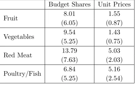
Table 1: Market Summary Statistics
Some simple market summary statistics are reported in Table 1. Each cell contains a
mean and standard deviation (in brackets). Taken altogether, fruit, vegetables, red meat,
and poultry/fish account for roughly 38 percent of a household’s monthly spending on food on
average. The largest share of the budget goes towards red meat, followed by vegetables, then
fruit, and finally poultry/fish. Furthermore, red meat and poultry/fish are more expensive
on average than fruit and vegetables. While these average descriptive statistics are meant to
provide a backdrop for the empirical analysis which follows, we should also note that there
is substantial heterogeneity in these data.
4.2 Rationalizability
We assume that food aggregates within the subgroup{fruit, vegetables}are weakly
sepa-rable from those within the subgroup{red meat, poultry/fish}, i.e., preferences over fruit and
vegetables are independent of the consumption of anything other than fruit and vegetables,
and similarly for red meat and poultry/fish. These assumptions are standard simplifications
in applied empirical work which allow us to focus our attentionwithin each subgroup, i.e., on
the interactionbetween fruit and vegetables andbetween red meat and poultry/fish. The
as-sumption is of course not beyond question since one can imagine complementarities existing
across subgroups. However, a decision-making procedure compatible with this assumption is
multi-stage budgeting, where the household first allocates an amount of expenditure to each
commodity group, and then chooses the consumption levels within each of these groups, i.e.,
meat and poultry/fish, and then decides how much of each to purchase.19
The assumptions stated above allow us to focus our analysis within each subgroup, i.e., we
are able to rest for rationalizability by utility maximization and additive separability within
the subgroups {fruit, vegetables} and {red meat, poultry/fish}. The first natural step in
the empirical analysis is to perform a series of exact tests. Only 14 out of 4,027 households
exhibit choice behavior that is consistent with the maximization of a stable preference over
fruit and vegetables, and among these, just 7 are consistent with additive separability. Rates
of rationalizability are similarly low for red meat and poultry/fish, with only 23 households
rationalizable by utility maximization, and 21 by additive separability.
These rates are exceptionally low, which is unsurprising given the sharpness of the exact
tests, which are applied to data sets containing 50 observations each. In order to proceed
empirically in a meaningful direction, it is necessary to take into account the distances or
departures from rationality, or in the language of econometrics, to allow for error terms. As
described in Section 3.4, following Halevy, Persitz, and Zrill (2016) and Polisson, Quah, and
Renou (2017), among others, we extend the notion of Afriat’s (1972, 1973) cost inefficiencies
to the additively separable case, which allows us to calculate a critical cost efficiency index
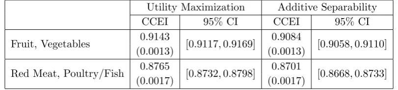
(CCEI) for both utility maximization and additive separability.20
Utility Maximization Additive Separability
CCEI 95% CI CCEI 95% CI
Fruit, Vegetables 0.9143 [0.9117,0.9169] 0.9084 [0.9058,0.9110]
(0.0013) (0.0013)
Red Meat, Poultry/Fish 0.8765 [0.8732,0.8798] 0.8701 [0.8668,0.8733]
[image:18.595.103.509.463.555.2](0.0017) (0.0017)
Table 2: Rationalizability Results
Some basic rationalizability results are displayed in Table 2. Each CCEI cell contains a
mean and standard error (in brackets), from which we then construct 95 percent confidence
intervals.21 For fruit and vegetables, the mean CCEI associated with utility maximization is
19 This procedure would, however, also require homotheticity within groups. See Gorman (1959). 20 Of course, the conventional econometric strategy is to introduce additive error terms to consumption
choices according to a minimum distance criterion. See Varian (1990) and Halevy, Persitz, and Zrill (2016) for a comparison of the revealed preference and distance based approaches.
about 0.9143, which means that the average household’s monthly budget needs to be reduced
by about 9 percent in order for the data to be rationalizable by utility maximization. In other
words, the average household is wasting about 9 percent of its monthly budget on fruit and
vegetables by departing from rationality in the form of utility maximization. A household’s
CCEI for additive separability isnecessarily going to be lower than for utility maximization,
which is due to the fact that additive separability is a more restrictive nested model. As
shown in Table 2, the mean CCEI for additive separability is 0.9084 for fruit and vegetables,
which is only moderately lower than 0.9143 in a meaningful economic sense. The pattern
is similar for red meat and poultry/fish, where the mean CCEI for utility maximization is
0.8765, and 0.8701 for additive separability.
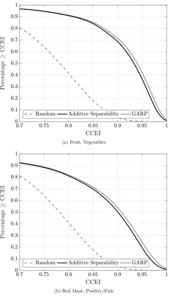
In order to examine the heterogeneity in CCEIs, we plot their distributions in Figure 4.
For fruit and vegetables, about 72 percent of households have a CCEI above 0.9 for utility
maximization, and about 91 percent have a CCEI above 0.8. In the additively separable case,
these figures are 69 and 91 percent at the 0.9 and 0.8 efficiency levels, respectively. What
emerges at first glance is that the data are largely rationalizable byboth utility maximization
and additive separability. In fact, the differences between the two models appear to be only
very slight; one might argue as before that these differences are not economically meaningful.
A similar story can be told for red meat and poultry/fish, where about 55 percent have a
CCEI above 0.9 for utility maximization, and about 82 percent have a CCEI above 0.8.
These figures are 51 percent and 81 percent at the 0.9 and 0.8 efficiency levels, respectively,
in the additively separable case. What also emerges is that rates of rationalizability for both
utility maximization and additive separability are lower within the subgroup {red meat,
poultry/fish} than {fruit, vegetables} at all efficiency levels.
While at first glance these results lend some support to both utility maximization and
additive separability as plausible modes of explanation, it is useful to make a comparison
to an alternative behavioral hypothesis. Following the convention in the empirical revealed
preference literature, we adopt as our alternative the ‘irrational consumer’ of Becker (1962),
who is naively choosing randomly uniformly from the frontiers of his budget sets. In our
(a) Fruit, Vegetables
[image:20.595.133.482.60.676.2](b) Red Meat, Poultry/Fish
procedure, we simulate data at the household level, first within the subgroup{fruit,
vegeta-bles} and then within the subgroup {red meat, poultry/fish}.22 The dashed gray lines in
Figures 4a and 4b correspond to the CCEI distributions for utility maximization among the
simulated households. Since the CCEI distributions for additive separability among the
sim-ulated households would be even lower than for utility maximization, the visual comparisons
in Figure 4 are conservative. The differences between our panel of British households and
their simulated ‘irrational’ counterparts are noticeably pronounced, again suggesting that
both utility maximization and additive separability provide considerable explanation.
While these basic rationalizability results are indeed suggestive, in the remaining three
subsections we formalize our empirical claims, also in a statistical sense. To do so, we
decompose the analysis into three parts, first focusing on pass rates, then on restrictive and
predictive power, and finally on a measure of predictive success which aggregates the two.
4.3 Pass Rates
It is natural to more deeply examine the performances of these models in terms of their
pass rates at different efficiency thresholds. For example, fixing the efficiency level at 0.95,
we can ask how many households are rationalizable by utility maximization or additive
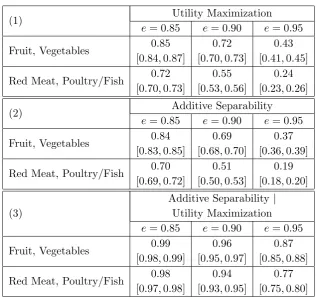
sep-arability, allowing for 5 percent cost inefficiency. Table 3 displays pass rates and exact 95%
confidence intervals for utility maximization and additive separability at the 0.85, 0.9, and
0.95 efficiency thresholds;23 panel (1) corresponds to utility maximization, panel (2) to
addi-tive separability, and panel (3) to addiaddi-tive separability conditional on utility maximization.
Notice that with so many households, all of these pass rates are very precisely estimated.
As shown in panels (1) and (2) of Table 3, our most basic empirical finding is that utility
maximization explains more of the data than additive separability,24 but only modestly.
22For example, within the subgroup{fruit, vegetables}, we generate a random sample of 100,000 simulated
or synthetic households, each of whom is choosing randomly uniformly from 50 budget lines. For each synthetic household, a set of 50 budgets is selected at random (and with equal probability) from among the 4,027 sets that have been observed in our sample (assuming that the sample is random and representative of the population). We conduct a similar exercise within the subgroup{red meat, poultry/fish}.
23At a given efficiency threshold, a household either passes or fails the test for a given model; the underlying
random variable is therefore Bernoulli distributed, and the sample pass rates are then binomially distributed. Confidence intervals areexact in the sense that they are obtained from the binomial distribution using the procedure first proposed by Clopper and Pearson (1934).
(1) Utility Maximization
e= 0.85 e= 0.90 e= 0.95
Fruit, Vegetables 0.85 0.72 0.43
[0.84,0.87] [0.70,0.73] [0.41,0.45]
Red Meat, Poultry/Fish 0.72 0.55 0.24 [0.70,0.73] [0.53,0.56] [0.23,0.26]
(2) Additive Separability
e= 0.85 e= 0.90 e= 0.95
Fruit, Vegetables 0.84 0.69 0.37
[0.83,0.85] [0.68,0.70] [0.36,0.39]
Red Meat, Poultry/Fish 0.70 0.51 0.19 [0.69,0.72] [0.50,0.53] [0.18,0.20]
(3)
Additive Separability|
Utility Maximization
e= 0.85 e= 0.90 e= 0.95
Fruit, Vegetables 0.99 0.96 0.87
[0.98,0.99] [0.95,0.97] [0.85,0.88]
[image:22.595.147.465.60.357.2]Red Meat, Poultry/Fish 0.98 0.94 0.77 [0.97,0.98] [0.93,0.95] [0.75,0.80]
Table 3: Pass Rates and 95% Confidence Intervals
For example, for fruit and vegetables, and at an efficiency threshold of 0.85, about 85%
of households are rationalizable by utility maximization, and 84% by additive separability;
furthermore, this difference is statistically significant at a 0.05 significance level.25 This
empirical finding, that utility maximization explains statistically more of the data than
additive separability, but only modestly, holds across both subgroups and all efficiency levels.
A second empirical finding, which is shown in panels (1) and (2) of Table 3, is that rates of
rationalizability for both utility maximizationand additive separability within the subgroup
{fruit, vegetables} are noticeably higher than their counterparts within the subgroup {red
meat, poultry/fish}, a statement which holds across efficiency thresholds, and which is also
statistically robust.26 It is of course natural to examine pass rates for additive separability
conditional on already being rationalizable by utility maximization; these are displayed in
than additive separability in terms of rationalizing the data.
25 If we observe a even single household that is rationalizable by utility maximization but not by additive
separability (which is nested within utility maximization), then the true pass rates cannot be equal.
26By statistically robust, we mean that a difference in pass rates (which are non-nested but realized within
panel (3) of Table 3. Within both subgroups, and across efficiency levels, these conditional
pass rates are very high; furthermore, they are modestly higher across efficiency thresholds
within the subgroup {fruit, vegetables}, and these differences are statistically significant.
4.4 Power
Rationalizability, be it exact or approximate (in terms of cost inefficiencies), only
mea-sures whether a given data set is consistent with utility maximization, additive separability,
or additive separability given utility maximization. These models, and their tests, can be
more or less observationally stringent, depending on both the theoretical structure in play
and the particular data which have been observed. Bronars (1987) proposed to measure the
power of a model/test as the probability that a consumer who is choosing randomly
uni-formly from his budget frontiers will fail the test for a given model. Since Bronars (1987),
it has become standard in applied empirical work in the revealed preference literature to
assess power in this way. In practice, we numerically approximate the power by simulating
data; we generate 100,000 synthetic data sets (as described in Section 4.2), and calculate the
fraction of these data sets which fail the tests for utility maximization and additive
separa-bility at specified efficiency thresholds.27 To numerically approximate the conditional power
of additive separability, we first fix an efficiency threshold, say 0.9, and generate 100,000
synthetic data sets (again as described in Section 4.2), which also obey GARP, i.e., which
are rationalizable by utility maximization in the first place.28
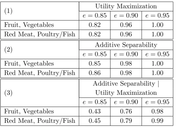
Table 4 displays the Bronars (1987) power measures for utility maximization and additive
separability at the 0.85, 0.9, and 0.95 efficiency thresholds; panel (1) again corresponds to
utility maximization, panel (2) to additive separability, and panel (3) to additive separability
conditional on utility maximization. As shown in panels (1) and (2) of Table 4, the
uncon-ditional power for both utility maximization and additive separability is very high, and this
holds within both subgroups and across efficiency thresholds. For example, for fruit and
27 It is clear from Hoeffding’s (1963) inequality (or by plotting the simulation results against the number
of simulations) that 100,000 random draws are sufficiently many to guarantee convergence.
28The conditional power procedure is slightly more complicated. For each synthetic household, a set of 50
(1) Utility Maximization
e= 0.85 e= 0.90 e= 0.95
Fruit, Vegetables 0.82 0.96 1.00 Red Meat, Poultry/Fish 0.82 0.96 1.00
(2) Additive Separability
e= 0.85 e= 0.90 e= 0.95
Fruit, Vegetables 0.85 0.98 1.00 Red Meat, Poultry/Fish 0.86 0.98 1.00
(3)
Additive Separability|
Utility Maximization
e= 0.85 e= 0.90 e= 0.95
[image:24.595.165.451.63.271.2]Fruit, Vegetables 0.43 0.76 0.98 Red Meat, Poultry/Fish 0.45 0.79 0.99
Table 4: Bronars Power
vegetables, and at an efficiency threshold of 0.85, about 18% of the simulated households
are rationalizable by utility maximization, and 15% by additive separability; naturally, the
power measures are greater still at higher efficiency thresholds. Furthermore, the differences
in power across the two subgroups appear only to be very slight, i.e., their unconditional
power is nearly identical at every efficiency threshold.
The conditional power of additive separability is shown in panel (3) of Table 4. Within
both subgroups, and across efficiency levels, these conditional measures are much lower
than in the unconditional case. For example, for fruit and vegetables, and at an efficiency
threshold of 0.85, about 57% of the simulated households which are already rationalizable
by utility maximization are subsequently rationalizeable by additive separability; as in the
unconditional case, the conditional power measures are greater at higher efficiency thresholds,
with nearly perfect power at the 0.95 efficiency threshold. Once again, the differences in
conditional power across the two subgroups appear only to be very slight.
Given that the unconditional power of both utility maximization and additive separability
is very high, and also that these power measures (both unconditional and conditional) exhibit
very little variation across subgroups, many of the conclusions that were drawn from the
investigation of basic pass rates in Section 4.3 would at first glance appear to be robust. We
4.5 Adjusted Pass Rates
While the empirical results (in terms of pass rates and power) presented so far suggest that
both utility maximization and additive separability have meaningful explanatory purchase
in these data, we require a more formal procedure in order to make a robust claim. To
this end, we appeal to an index of predictive success first proposed by Selten (1991). The
Selten index aggregates two components: (1) the relative frequency of correct predictions,
i.e., the ‘hit rate’ which is equal to the pass rate, and (2) the relative size of the set of
predicted outcomes, i.e., the ‘imprecision’ which is equal to one minus the power. Selten
(1991) shows that a simple difference between the two obeys several desirable axiomatic
properties,29and subsequently proves that this index cannot be improved upon by any other
measure of predictive success which takes into account the same information.30 Building
upon Bronars (1987), Beatty and Crawford (2011) introduced the Selten index into the
revealed preference literature, and it has since been adopted widely in empirical work. The
essence of the approach is to mitigate the success of model in making correct predictions with
the (im)precision of those predictions, i.e., to adjust pass rates in light of power/precision.
As such, we refer to the Selten index of predictive success as an adjusted pass rate.
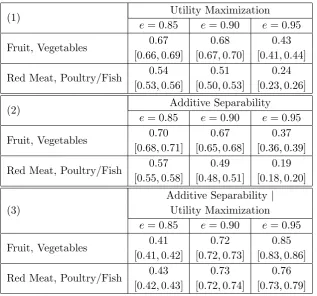
Table 5 displays the adjusted pass rates, or Selten indices of predictive success, and
95% confidence intervals (obtained from a bootstrap) for utility maximization and additive
separability across efficiency thresholds;31 panels (1)–(3) correspond to utility maximization
and additive separability (conditional on utility maximization) as in Tables 3 and 4. The first
observation is that all models, both unconditionally and conditionally, and across efficiency
thresholds, have positive predictive success which is statistically different from zero.32 In
29The Selten index satisfies three axioms: (1) monotonicity, i.e., passing a perfectly stringent test is better
than failing a perfectly lenient test; (2) equivalence, i.e., passing a perfectly lenient test is no more or less informative than failing a perfectly stringent test; and (3) aggregability, i.e., the measure can be aggregated across members of a heterogeneous sample, which is of course important in empirical work.
30 To be precise, any other measure of predictive success which obeys the same set of axioms must be an
affine transformation of this simple difference.
31 Notice that the adjusted pass rates are equal to the pass rates minus the imprecision, where the latter
is equal to one minus the power (see Section 4.4). Since power has been obtained numerically, we appeal to a simple bootstrap, i.e., a resampling (106 samples) of adjusted pass rates with replacement, in order to
obtain standard errors and confidence intervals.
32 To make this statement, we use bootstrapped standard errors in order to perform a t-test of the null
(1) Utility Maximization
e= 0.85 e= 0.90 e= 0.95
Fruit, Vegetables 0.67 0.68 0.43
[0.66,0.69] [0.67,0.70] [0.41,0.44]
Red Meat, Poultry/Fish 0.54 0.51 0.24 [0.53,0.56] [0.50,0.53] [0.23,0.26]
(2) Additive Separability
e= 0.85 e= 0.90 e= 0.95
Fruit, Vegetables 0.70 0.67 0.37
[0.68,0.71] [0.65,0.68] [0.36,0.39]
Red Meat, Poultry/Fish 0.57 0.49 0.19 [0.55,0.58] [0.48,0.51] [0.18,0.20]
(3)
Additive Separability|
Utility Maximization
e= 0.85 e= 0.90 e= 0.95
Fruit, Vegetables 0.41 0.72 0.85
[0.41,0.42] [0.72,0.73] [0.83,0.86]
[image:26.595.149.467.63.359.2]Red Meat, Poultry/Fish 0.43 0.73 0.76 [0.42,0.43] [0.72,0.74] [0.73,0.79]
Table 5: Adjusted Pass Rates and 95% Confidence Intervals
other words, the ability of these models to explain the data remains high, even after making
adjustments for power/precision.
From Section 4.3, our most basic empirical finding was that utility maximization
ex-plains more of the data than additive separability, but only modestly, and that these
differ-ences are statistically significant; such a claim can be moderated further after adjusting for
power/precision. The adjusted gaps (shown in panels (1) and (2) of Table 5) are narrower
than the unadjusted gaps (shown in panels (1) and (2) of Table 3), and in some cases (at the
0.85 efficiency threshold) the direction is reversed, and all differences are statistically
signif-icant at a 0.05 significance level. Our primary empirical finding from Section 4.3 was that
the rates of rationalizability for both utility maximization and additive separability are
sub-stantively (and statistically) higher within the subgroup{fruit, vegetables} than{red meat,
poultry/fish}; this finding holds (statistically) even after adjusting for power/precision (see
again panels (1) and (2) of Table 5). Lastly, the adjusted conditional pass rates (shown in
(3) of Table 3), although they remain (statistically) greater than zero. Furthermore, the
adjusted pass rates are substantially higher within the subgroup {fruit, vegetables} than
{red meat, poultry/fish} at the 0.95 efficiency threshold (suggesting greater
substitutabil-ity/complementarity within the latter subgroup), and only modestly lower at the 0.85
effi-ciency threshold; these differences are statistically significant at a 0.05 significance level.33
5. Conclusions
In this paper, we develop and implement a nonparametric lattice test for additive
separa-bility. While this preference structure is commonly used to simplify the analysis of consumer
choice, it has long been thought that it imposes unreasonable restrictions on observable data,
i.e., “the price [of additivity] is too high”. The lattice approach, which is purely
nonpara-metric and applied to finite data, suggests that perhaps the empirical price of additivity is
not as high as it might first appear. Future work could extend the approach developed in
this paper to new and different empirical settings with little difficulty.
Appendix A
A.1 Concave Additive Separability
Suppose that `goods are divided into two groups, and that there are `1 goods in group 1
and`2 goods in group 2, so that`1+`2 =`. Now the data set{(pt, xt)}Tt=1 can be partitioned
into two subsets {(qt, yt)}T
t=1 and {(rt, zt)}Tt=1, which correspond to groups 1 and 2.34 Definition 7. The data set {(pt, xt)}Tt=1, which can be partitioned into the two subsets
{(qt, yt)}T
t=1 and {(rt, zt)}Tt=1, is rationalizable by concave additive separability if there exist
increasing, concave, and continuous utility functions v : R`1
+ → R and w : R`+2 → R, such
that, at every observation t= 1,2, . . . , T,
v(yt) +w(zt)>v(y) +w(z) for any x= (y, z)∈ {x∈R`
+ :p
t·x
6pt·xt}.
Theorem 3. The following statements are equivalent:
33 There is no statistical difference between the two subgroups at the 0.90 efficiency threshold. 34 Notice thatyt∈
R`+1,zt∈R
`2
+, qt∈R
`1
++, andrt∈R
`2
++, so thatxt= (yt, zt) andpt= (qt, rt) for all
1. The data set {(pt, xt)}T
t=1, which can be partitioned into the two subsets {(qt, yt)}Tt=1
and {(rt, zt)}T
t=1, is rationalizable by concave additive separability.
2. For the data set{(pt, xt)}T
t=1, which can be partitioned into the two subsets {(qt, yt)}Tt=1
and {(rt, zt)}T
t=1, at every observation t = 1,2, . . . , T, there exist numbers vt, wt ∈ R
and λt ∈
R++, such that
vt0 6vt+λtqt·(yt0 −yt) for all t, t0 = 1,2, . . . , T, (V1)
wt0 6wt+λtrt·(zt0 −zt) for all t, t0 = 1,2, . . . , T. (V2)
Proof of Theorem 3. (1) =⇒ (2): If the data set {(pt, xt)}T
t=1, which can be partitioned
into the two subsets {(qt, yt)}T
t=1 and {(rt, zt)}Tt=1, is rationalizable by concave additive
sep-arability, then at every observation t = 1,2, . . . , T, there exists a number λt ∈ R++, such
that λtqt ∈∂v(yt) and λtrt ∈∂w(zt) for all t = 1,2, . . . , T, where∂v(yt) and ∂w(zt) denote
the super-differentials of v and wevaluated at yt and zt. Notice that the elements of ∂v(yt) and ∂w(zt) are positive sincev and ware increasing. Given the concavity of v and w,
v(yt0)6v(yt) +∂v(yt)·(yt0 −yt) for all t, t0 = 1,2, . . . , T,
w(zt0)6w(zt) +∂w(zt)·(zt0−zt) for all t, t0 = 1,2, . . . , T.
Together with the first-order conditions, the above inequalities imply that at every
observa-tion t= 1,2, . . . , T, there exists a numberλt ∈R++, such that
v(yt0)6v(yt) +λtqt·(yt0 −yt) for all t, t0 = 1,2, . . . , T,
w(zt0)6w(zt) +λtrt·(zt0−zt) for all t, t0 = 1,2, . . . , T.
Letting vt = v(yt) and wt =w(zt) for all t = 1,2, . . . , T, implies that at every observation
t= 1,2, . . . , T, there exist numbers vt, wt∈
Rand λt∈R++, such that (V1) and (V2) hold.
(2) =⇒ (1): Given the data set {(pt, xt)}T
t=1, which can be partitioned into the two
subsets {(qt, yt)}T
t=1 and {(rt, zt)}Tt=1, if, at every observation t = 1,2, . . . , T, there exist
numbers vt, wt∈
R and λt∈R++, such that (V1) and (V2) hold, then for any y∈R`+1 and
z ∈R`2
+, define the functionsv :R
`1
+ →R and w:R
`2
+ →R according to
v(y) = min
t {v
w(z) = min
t {w
t+λtrt·(z−zt)}.
Notice that v and w are increasing, concave, and continuous. By the definitions ofv and w,
v(yt) = vm+λmqm·(yt−ym)6vt+λtqt·(yt−yt) =vt for all t= 1,2, . . . , T,
w(zt) =wn+λnrn·(zt−zn)6wt+λtrt·(zt−zt) =wt for all t= 1,2, . . . , T,
for somemandn, which hold with equality in order not to violate (V1) and (V2). Therefore,
v(yt) = vt and w(zt) =wt for allt = 1,2, . . . , T. At any observation t = 1,2, . . . , T, choose
some x= (y, z)∈ {x∈R`
+ :pt·x6pt·xt}. Again by the definitions ofv and w,
v(y)6vt+λtqt·(y−yt),
w(z)6wt+λtrt·(z−zt).
Summing the above inequalities implies that
v(y) +w(z)6vt+wt+λtqt·(y−yt) +λtrt·(z−zt) =vt+wt+λtpt·(x−xt)
6vt+wt
=v(yt) +w(zt).
A.2 Proof of Theorem 2
The proof of Theorem 2 makes use of the following lemma.
Lemma 1. Let {(xt,Ct)}Tt=1 denote a finite set of observations drawn on an individual
con-sumer, where xt ∈ R`
+ corresponds to the consumption bundle chosen from the constraint
set Ct ⊂
R`+ at every observation t = 1,2, . . . , T. Further suppose that each Ct is compact
and downward closed, i.e., for any x ∈ Ct and y ∈
R`+, if y < x, then y ∈ Ct.35 Let ∂Ct
denote the upper boundary of Ct, i.e., x ∈ ∂Ct if there is no y ∈ Ct such that y > x, and
assume that xt ∈ ∂Ct for all t = 1,2, . . . , T. If there is a finite collection of sets {X i}`i=1,
35 For anyx, y ∈
R`+, we say thatx>y ifxi >yi for all i= 1,2, . . . , `, that x > y ifx>y andx6=y,
where each finite set Xi ={x∈R+ :x=xti for some t} ∪ {0} for all i= 1,2, . . . , `, a finite
lattice L = Q`
i=1Xi, and a finite collection of functions {v¯i}
`
i=1, where each ¯vi : Xi → R is
increasing for all i= 1,2, . . . , `, such that, at every observation t= 1,2, . . . , T,
`
X
i=1
¯
vi(xti)> `
X
i=1
¯
vi(xi) for all x∈ Ct∩ L,
`
X
i=1
¯
vi(xti)> `
X
i=1
¯
vi(xi) for all x∈(Ct/∂Ct)∩ L,
then there is a finite collection of functions {vi}`i=1, where each vi : R+ → R is increasing
and continuous for all i= 1,2, . . . , `, such that, at every observation t= 1,2, . . . , T,
`
X
i=1
vi(xti)> `
X
i=1
vi(xi) for all x∈ Ct.
Proof. For eachi= 1,2, . . . , `, order the finite setXi so thatXi ={z0i, z1i, z2i, . . . , z Ki−1
i , z Ki
i },
where z0
i = 0 < zi1 < zi2 < · · · < z Ki−1
i < z Ki
i . For each i = 1,2, . . . , `, define the function
vi :R+ →R according to
vi(z) =
¯
vi(zi0) +
1
i
∆z1
i
(z−z0
i) for z ∈[zi0, zi1−1i]
¯
vi(zi1) +
∆¯v1
i
1
i
(z−zi1) for z ∈[zi1−1i, zi1]
¯
vi(zi1) +
2i
∆z2
i
(z−zi1) for z ∈[zi1, zi2−2i]
¯
vi(zi2) +
∆¯vi2 2
i
(z−z2
i) for z ∈[zi2−2i, zi2]
· · · for · · ·
¯
vi(zKi
−1
i ) +
Ki
i
∆zKi
i
(z−zKi−1
i ) for z ∈[z
Ki−1
i , z Ki
i − Ki
i ]
¯
vi(ziKi) +
∆¯vKi
i
Ki
i
(z−zKi
i ) for z ∈[z Ki
i − Ki
i , z Ki
i ]
¯
vi(ziKi) + Ki+1
i (z−z Ki
i ) for z ∈[z Ki
i ,+∞)
,
for some suitable vector i = (1i, 2i, . . . , Ki−1
i , Ki
i , Ki+1
i )0, where ∆zik= (zik−z k−1
i )−ki
and ∆¯vki = (¯vi(zik)−¯vi(zik−1))− k
and that, at every observation t= 1,2, . . . , T,
`
X
i=1
vi(xti)> `
X
i=1
vi(xi) for all x∈ Ct.
Suppose, to the contrary, that no choice of {i}`i=1 satisfies the above requirements, i.e., for
every choice of {i}`i=1, at some observationt,
`
X
i=1
vi(xti)< `
X
i=1
vi(xi) for some x∈ Ct.
Therefore, it must be the case that at some observation t,
`
X
i=1
¯
vi(xti) = `
X
i=1
vi(xti)
<
`
X
i=1
vi(xi)
=
`
X
i=1
¯
vi(yi) +δ({i}`i=1),
for some x ∈ Ct and somey ∈ Ct∩ Lor y ∈(Ct/∂Ct)∩ L, with y
6x; since {i}`i=1 can be
chosen in order to make δ({i}`i=1)>0 sufficiently small, this can only be true when
`
X
i=1
¯
vi(xti)< `
X
i=1
¯
vi(yi) for some y∈ Ct∩ L,
in the case where y∈ Ct∩ L, or when `
X
i=1
¯
vi(xti) = `
X
i=1
¯
vi(yi) for some y∈(Ct/∂Ct)∩ L,
in the case where y∈(Ct/∂Ct)∩ L. And so we have a contradiction.
Proof of Theorem 2. (1) =⇒ (2): If the data set {(pt, xt)}T
t=1 is rationalizable by additive
separability, then for eachi= 1,2, . . . , `, let ¯vi(xti) =vi(xti) for all t= 1,2, . . . , T.
(2) =⇒ (1): Given the data set {(pt, xt)}T
t=1, if there exist numbers ¯vi(xi)∈R for each
xi ∈ Xi = {x ∈ R+ : x = xti for some t} ∪ {0} for all i = 1,2, . . . , `, with ¯vi(xi) > v¯i(yi)
whenever xi > yi for any xi, yi ∈ Xi, such that (A1) and (A2) hold at every observation
References
AFRIAT, S. N. (1967): “The Construction of Utility Functions from Expenditure Data,” Inter-national Economic Review, 8(1), 67–77.
AFRIAT, S. N. (1972): “Efficiency Estimation of Production Functions,”International Economic Review, 13(3), 568–598.
AFRIAT, S. N. (1973): “On a System of Inequalities in Demand Analysis: An Extension of the Classical Method,”International Economic Review, 14(2), 460–472.
BEATTY, T. K. M., and I. A. CRAWFORD (2011): “How Demanding Is the Revealed Preference Approach to Demand?,”American Economic Review, 101(6), 2782–2795.
BECKER, G. S. (1962): “Irrational Behavior and Economic Theory,”Journal of Political Econ-omy, 70(1), 1–13.
BLACKORBY, C., D. PRIMONT, and R. R. RUSSELL (1978): Duality, Separability, and Func-tional Structure: Theory and Economic Applications. Amsterdam: North Holland.
BLUNDELL, R. (1988): “Consumer Behaviour: Theory and Empirical Evidence—A Survey,”
Economic Journal, 98(389): 16–65.
BRONARS, S. G. (1987): “The Power of Nonparametric Tests of Preference Maximization,”
Econometrica, 55(3), 693–698.
CHAMBERS, C. P., and F. ECHENIQUE (2016): Revealed Preference Theory. Cambridge: Cambridge University Press.
CHERCHYE, L., T. DEMUYNCK, B. DE ROCK, and P. HJERTSTRAND (2015): “Revealed Preference Tests for Weak Separability: An Integer Programming Approach,” Journal of Econometrics, 186(1), 129–141.
CLOPPER, C. J., and E. S. PEARSON (1934): “The Use of Confidence or Fiducial Limits Illustrated in the Case of the Binomial,”Biometrika, 26(4), 404–413.
CRAWFORD, I., and B. DE ROCK (2014): “Empirical Revealed Preference,” Annual Reviews, 6, 503–524.
CRAWFORD, I., and M. POLISSON (2016): “Demand Analysis with Partially Observed Prices,”
Discussion Papers in Economics, 15/12, University of Leicester.
DEATON, A. (1974): “A Reconsideration of the Empirical Implications of Additive Preferences,”
Economic Journal, 84(334), 338–348.
DEATON, A., and J. MUELLBAUER (1980): Economics and Consumer Behavior. Cambridge: Cambridge University Press.
DEBREU, G. (1960): “Topological Methods in Cardinal Utility Theory,” inMathematical Methods in the Social Sciences, 1959, ed. by K. J. Arrow, S. Karlin, and P. Suppes. Stanford: Stanford University Press.