Fore Body Side Vortex of KVLCC2 at 30° Drift: A Trailing Vortex Resolved with DES and Compared to PIV Data

(1)

https://www.scirp.org/journal/ojfd ISSN Online: 2165-3860

ISSN Print: 2165-3852

DOI: 10.4236/ojfd.2019.94020 Oct. 30, 2019 303 Open Journal of Fluid Dynamics

Fore-Body Side Vortex of KVLCC2 at 30˚ Drift:

A Trailing Vortex Resolved with DES and

Compared to PIV Data

Dag-Frederik Feder

*

, Ivan Shevchuk, Ahmed Sahab, Lukas Gerwers, Moustafa Abdel-Maksoud

FDS/TUHH, Hamburg, Germany

Abstract

A hybrid RANS-LES approach is used to resolve the Fore-body Side Vortex (FSV) separating from the KVLCC2 hull at 30˚ drift angle and Reynolds number 2.56 6

oa L

Re ≈ e . The performance of the DES approach is evaluated

using a proper grid study. Besides, the following aspects of the CFD results are investigated: the resolution of turbulent energy, the prediction of in-stantaneous and time-averaged vortical structures, local flow features, the limiting streamlines and the evolution of the vortex core flow. New PIV da-ta from wind tunnel experiments is compared to the latter. The results form a basis for future investigations in particular on the vortex interaction fur-ther downstream and the applicability of different kinds of turbulence models to trailing vortices like the FSV. Turbulence modelling is realised with the k-ω-SST-IDDES model presented in [1], the grids’ cell count is 6.4 M, 10.5 M and 17.5 M. Grid convergence of the time-averaged vortex core flow is ob-served. OpenFOAM version 1806 is used to carry out the simulations and snappyHexMesh to build the mesh.

Keywords

KVLCC2, DES, Hybrid RANS-LES, PIV, Trailing Vortex, Drift

1. Introduction

Coherent vortices occur for example as wing tip vortices. Several test cases have been investigated including e.g. [2] and [3]. Here we refer only to the experi-mental investigations as there are numerous publications on CFD validation stu-dies. These coherent vortices trail downstream of a foil’s trailing edge as the free shear layer rolls up. As observed e.g. in the experimental studies, the decay is How to cite this paper: Feder, D.-F.,

Shevchuk, I., Sahab, A., Gerwers, L. and Abdel-Maksoud, M. (2019) Fore-Body Side Vortex of KVLCC2 at 30˚ Drift: A Trailing Vortex Resolved with DES and Compared to PIV Data. Open Journal of Fluid Dynam-ics, 9, 303-325.

https://doi.org/10.4236/ojfd.2019.94020

Received: July 19, 2019 Accepted: October 27, 2019 Published: October 30, 2019

http://creativecommons.org/licenses/by/4.0/

(2)

DOI: 10.4236/ojfd.2019.94020 304 Open Journal of Fluid Dynamics

very slow, e.g. in [3], the peak tangential velocity and the viscous core diameter are smeared out very little over 30 times the chord length downstream. A possi-ble explanation for the persistency is the relaminarisation that occurs inside the viscous core.

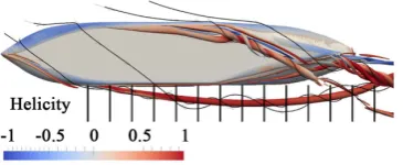
The Fore-body Side Vortex (FSV) analysed in the following, see Figure 1, is also a trailing vortex but not downstream of the lift-generating body. It is conti-nuously fed by the roll-up of the separating boundary layer, the free shear layer. As the FSV is located inside the separation zone, the turbulent energy is expected to be high. To properly resolve this flow, a hybrid RANS-LES approach is un-dertaken here: the near-wall turbulent flow is modelled with RANS and the out-er flow, e.g. the vortex, is resolved. Motivated by previous work on this case at the institute, see [4], the numerical setup and modelling approach is updated. An overview is presented at the end of this section.

Although there are similarities to wing tip vortices the following literature re-view focuses mainly on research on this vortical structure to consider the find-ings on turbulence models, etc. The authors analysed the influence of different turbulence modelling approaches and different grid types and sizes on the for-mation of the complex vortex system in the near wake of the hull.

The KVLCC2 hull and its modified versions like KVLCC2M have been inves-tigated in several workshops: Gothenburg 2000 [5] and 2010 [6][7][8], Tokyo 2005 [9] and SIMMAN 2008 [10] [11]. The following papers follow on these workshops.

Fureby et al.[12] conducted simulations using RANS, DES and LES for 0, 12 and 30˚ drift angle with three CFD codes. Grids with a cell count from 13 M to 202 M were used. Vortex instabilities were investigated. Furthermore, vortex structures, the flow at the propeller plane and limiting streamlines were ana-lysed.

(a)

[image:2.595.256.488.487.656.2]

(b)

Figure 1. KVLCC2 at 30˚ drift angle with vortices. Isosurfaces both coloured by norma-lized helicity. (a) Qualitative view of the vortex system and selected streamlines. The plane A-A indicates an exemplary measuring plane for the analysis of the FSV; (b) Evolu-tion of the FSV on the medium mesh with isosurface 2 2

100

pp

QL U∞= (based on time-averaged

(3)

Abdel-Maksoud et al.[4] presented experimental results obtained in TUHH’s wind tunnel and CFD results from five partners for 30˚ drift angle. Experi-mental data was obtained by smoke tests for the global vortex structure, oil film tests for the limiting streamlines and PIV investigations on different vor-tices. Turbulence modelling ranges from linear eddy-viscosity RANS models up to hybrid RANS-LES models. Finally the authors concluded that no turbulence model provided satisfactory results for all aspects of the flow. The results were analysed in a different coordinate system aligned to the wind tunnel test section, hence a comparison of the x-component of velocity or vorticity is difficult for the current approach.

Xing and colleagues [13][14] performed simulations at 0, 12 and 30˚ drift an-gle with Explicit Algebraic Reynolds Stress Models (EARSM) and DES based on the EARSM on a mesh with 13 M cells. The focus is put on the development of the different coherent vortices in the wake including an analysis of vortex breakdown and helical instability of the initial FSV. This includes an analysis of the TKE budget, so the terms in the differential equation for modelled TKE. Be-sides, the hull forces, the limiting streamlines, the flow at the propeller plane and the flow at the vortex core line is investigated. The underlying mesh is aligned to the inflow; this is the reason why the axial velocity and vorticity component are parallel to the flow. Within the present paper, the axial components are aligned to the ship’s longitudinal axis and therewith approximately parallel to the axis of the FSV.

Ismail et al. [15] put the focus on high-order convection schemes to reduce the influence of numerical diffusion using isotropic and anisotropic Reynolds stress models and DES. Abbas et al. performed RANS and hybrid simulations for 0 and 12˚ drift angle. They noticed issues with the SAIDDES model in the stern area due to erroneous flow separation.

The present approach is based on scale resolving simulations applying the k-ω-SST-IDDES model presented in [1]. The results provide a basis for future investigations mainly on the vortex interaction in the stern wake and the appli-cability of different kinds of turbulence models to trailing vortices. Here, the be-haviour of the DES technique is presented: the resolution of vortical structures in the instantaneous flow field, the resolution of turbulent energy, the switch from RANS to LES and the evolution of the flow at the vortex core line. New PIV data from wind tunnel experiments is compared to the latter. The data is obtained in the institute’s wind tunnel as succeeding investigations of [4].

(4)

2. Case Description

Vortex system and FSV The flow around the KVLCC2 hull at a drift angle of 30˚ and at the Reynolds number 2.56 6

oa L

Re ≈ e is simulated with special focus

on the coherent leeward vortex. Figure 1 shows the vortex system in the wake with several coherent structures interacting. Within this paper the focus is put on the fore-body side vortex (FSV) which develops for a certain distance without the influence of other vortices. While the FSV trails downstream is fed by the separating free shear layer that rolls up around its core.

The ASV separates on the windward side of the hull and develops close to the hull’s bottom in the boundary layer. Near the ship’s stern several small and large vortices (AHPV, SV and ABV) separate and interact further downstream. The hull’s wake is dominated by this interaction which creates a much more complex flow field than upstream where the FSV evolves separately.

Flow parameters The inflow conditions are presented in Table 1. To avoid any vibration of the model due to unsteady forces induced by the separation re-gions the uniform inflow velocity is reduced from 27 m/s in [4] to 25 m/s. As the free shear layer separates at the bilge and the FSV is continuously fed by the roll up, no turbulence generator is used because sufficient flow instabilities are as-sumed to be generated.

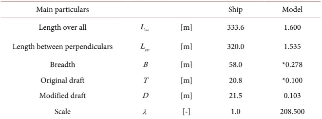
KVLCC2 model geometry The KVLCC2 hull introduced in [16] is consi-dered in the CFD investigations and placed in the wind tunnel test section. It has a low Froude number bulbous bow shape. A double-body model of the under-water hull of KVLCC2 is used for the experimental investigations in the wind tunnel in [4]. The CAD-data of the hull is mirrored about the waterline, which is located at the modified draft D. Compared with the original draft of the ship; the draft of the investigated model is increased in order to avoid a strong disconti-nuity of the hull near the forward perpendicular. The propeller hub is closed by a half-sphere. The main dimensions of the ship and model are given in Figure 2 and Table 2.

[image:4.595.271.477.586.669.2]

A double-body model is placed in the wind tunnel but flow simulations are carried out for a single hull. Both approaches realise a symmetry boundary con-dition at the imaginary waterline. For CFD this is realised with a slip or zero- gradient boundary condition.

Figure 2. Side view of KVLCC2 as double body model with forward perpendicular (FP), after perpendicular (AP), L_oa,L_pp and distance between transom stern and FP (in [mm]).

(5)

[image:5.595.209.539.91.141.2]

DOI: 10.4236/ojfd.2019.94020 307 Open Journal of Fluid Dynamics Table 1. Inflow properties at the wind tunnel test section.

Inflow velocity U∞ _temperatureAir Viscosity _ν Density ρ ReLoa

2 3 I= k U∞

25 m/s ≈23˚C 1.56e-5 m2_/s _{1.19 kg/m}3 _≈2.56e6 _0.3%

Table 2. Dimensions of KVLCC2 model (model scale values are rounded to millimeters). There is a typo for the values marked with * in [1].

Main particulars Ship Model

Length over all Loa [m] 333.6 1.600

Length between perpendiculars Lpp [m] 320.0 1.535

Breadth B [m] 58.0 *0.278

Original draft T [m] 20.8 *0.100 Modified draft D [m] 21.5 0.103

Scale λ [-] 1.0 208.500

The Cartesian coordinate system is aligned to the ship model’s longitudinal axis: The x-axis points towards the stern, the y-axis in the portside direction and the z-axis towards the ships bottom (perpendicular to the inflow).

3. Experimental Setup

As this investigation succeeds the one presented in [4], the experimental setup in the wind tunnel is similar, differences are listed below:

 _{Different inflow conditions (speed/Reynolds number);}  _{Different orientation and location of the measurement planes;}

 New coordinate system aligned to the new measurement planes. This is im-portant as the velocity and vorticity component normal to the planes are analysed.

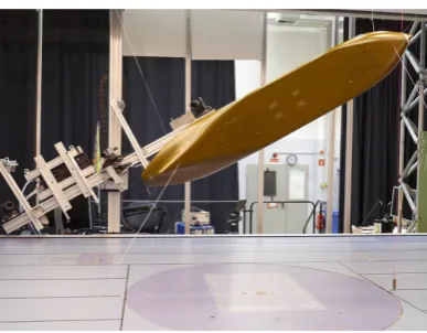
Wind tunnel The TUHH low-speed wind tunnel (Figure 3) of the Institute for Fluid Dynamics and Ship Theory (FDS) provides an outstanding facility for investigating the aerodynamic characteristics of ship super-structures as well as for investigating the hydrodynamics of subsurface objects and the underwater hull of common ships. The main technical specifications of the wind tunnel are summarized in Table 3. The wind tunnel can be operated in either a closed or an open loop mode. Velocity measurements by PIV are performed at the closed loop mode.

The test section allows manual and optical access from the top and the lateral sides. Positioning the PIV measurement system is supported by a multiple-axes traversing system mounted to the lateral sides of the section, thus allowing the measurement of the flow velocity at various planes and positions.

[image:5.595.209.540.185.307.2]

(6)

[image:6.595.211.539.70.206.2] [image:6.595.212.538.72.359.2]

DOI: 10.4236/ojfd.2019.94020 308 Open Journal of Fluid Dynamics Figure 3. Wind tunnel at TUHH.

[image:6.595.277.471.238.389.2]

Figure 4. Model and PIV system in the test section.

Table 3. Wind tunnel of the institute for fluid dynamics and ship theory at TUHH: main particulars.

Dimensions of the test section Length 5.5 m Width 3 m Height 2 m

Max. velocity 35 m/s

Contraction ratio nozzle 4.125

Fan unit power 400 kW

perpendicular (FP) is about 1.93 m and the distance between the wind tunnel bottom and the line which represents the intersection between the double-body symmetry plane and the transom stern is about 0.50 m (values rounded to [cm]). The model is placed in the middle of the test section width, hence the “bounda-ries” of the open test section are located at zW = = ±z 1.5 m. The model is

sus-pended inside the test section by 8 wires, each 1.0 mm in diameter. The forward and the aft four wires are fixed at

x L

_pp

=

0.085

and at

x L

_pp

=

0.908

,

respec-tively. Figure 4 shows the PIV system aligned to the inclined model in the test section.

[image:6.595.208.540.455.544.2]

(7)

2.5% of Loa. The blockage factor (ratio between the projected areas of the double

model and the cross section of the measuring section) is about 0.026. In the for-ward region of the model, the leefor-ward side is close to the wind tunnel ceiling. In the aft region, the windward side comes close to the wind tunnel bottom. The sidewalls of the test section are open and the ceiling and the bottom are closed during the tests. Due to these special blockage conditions, the velocity deviations in the far field of the model are about 1% of the adjusted inflow wind speed.

[image:7.595.284.467.633.708.2]

Measuring planes Within the current measurements, PIV data has been ob-tained for planes parallel to ship frames (y-z-planes). The reason for this choice of the plane orientation is that the flow in the model wake is mostly parallel to the hull walls, hence is normal to the measurement planes. So e.g. the axis of the large fore-body side vortex (FSV) is (nearly) orthogonal to the planes and follow-ing its axial vorticity can be determined. (This is valid until the FSV bends to-wards the symmetry plane.) The fact that the FSV is almost perpendicular to the ship frames is also the reason for the introduction of the new coordinate system.

Figure 5 shows the measuring planes with a distance of 0.1 m each, the exact positions are:

[ ]

_m _{0.361, 0.461,} _{,1.561 ,1.661}*

x =   _

this corresponds to (rounded values)

*

0.235, 0.300, ,1.017 ,1.082 .

pp

x L =   _

The measurement plane at the transom stern is marked with *. The following data is available from the experiments for each plane:

 velocity (vector field:

U U U

_x

,

_y

,

_z);

 vorticity normal to the planes (scalar field:

ω

x).

PIV system The spatial distribution of the velocity components in different planes is measured by a modular commercial 2D-3C-PIV system of TSI Inc. The stereoscopic PIV system (SPIV) consists of a pulsed laser, light sheet optics, two cameras, a synchronizer and a computer with software to control image genera-tion and processing.

The light sheet is generated by a 200 mJ two-head Nd-YAG-laser (Quantel Big Sky) and the light sheet optics. Scattered light is received by two PowerView 4 M (2048 × 2048 pixel, 12 bit, monochrome) cameras equipped with Nikon 300 mm f/4D AF-S lenses; their baseline is located approximately 1.7 m from the middle of the test section and positioned on both sides of the laser plane. Six measur-ing planes at each measurmeasur-ing station were investigated. The planes are arranged

(8)

in 2 × 3 configuration, where two planes are measured beside each other in y-direction and 3 planes are measured above each other in z-direction. The overlap between neighbouring planes is 50%. The optical axes of the lenses are inclined 27.5˚ and 24.5˚ to the normal of the laser plane for the middle planes and ±0.5˚ for the other planes. At capture frequency of 7.25 Hz, 1000 images were recorded at each measuring plane.

In order to avoid blur caused by the oblique view of the cameras, a rotatable base adjusts the angle between the lens and CCD chip to satisfy Scheimpflug condition. The cameras record two images each with a short time separation (∆ =T 15 sµ ). In order to reach sufficient signal-to-noise ratio for the

subse-quent image processing and to minimize the loss of particle pairs, the time sepa-ration was selected to meet the condition that a particle would travel more than 25% of the light sheet thickness.

For the PIV measurements, particles of an average diameter of about 1 μm are generated as the seeding. The Laskin type droplet generator uses dioctyl sebacate (DOS). The generator is placed downstream of the test section. The fog generat-ed spreads through the wind tunnel at a closgenerat-ed loop operational mode and leads to a global seeding. Therefore, any influence due to turbulence of the generated fog is negligible.

The images was analysed by means of a FFT-transformation, cross correlation technique and ensemble averaging of the calculated correlation maps. Gaussian curve fitting was applied to estimate the location of the correlation peak with sub-pixel accuracy. No pixel locking effects were recognized. The results were calculated with a 50% overlap of neighbouring vectors for the two-component vector maps of each camera. Reconstruction of three component velocities is based upon the vector maps of both cameras as well as calibration data.

The calibration is executed by capturing a set of images for a calibration target. A black calibration target with a predefined rectangular grid of dots spread on two planes was used to capture the calibration images. The required calibration data was calculated by evaluating these images. The calibration of the PIV sys-tem is sensitive to even small changes of the geometrical and optical configura-tion. Therefore, the whole PIV-components were installed on one crossbar. Then the crossbar can be moved by the traversing mechanism in vertical and horizontal direction.

Data reduction The velocity components are calculated by using the full set of data. In order to calculate the velocity fluctuation, the set of data is divided into 20 smaller packs of 50 images each. For comparison reasons, the same in-vestigation was conducted with 10 packs of 100 images each, 50 packs of 20 im-ages each and 100 packs with 10 imim-ages each. The velocity components Ui are

computed using:

, 1

1 N

i i k

k

U U

N =

=

∑

₍₁₎

(9)

represents the collected data for every interrogation area. The differentials of the velocity components are used to compute the vorticity vector components ac-cording to its definition as the rotation of the velocity field.

Uncertainty assessment The PIV system was mounted on a crossbar, 2D au-tomated traverse system. The uncertainty of the positioning is ±0.1 mm. The es-timated uncertainties of the three velocity components according to prior mea-surements with the same configuration are W = ±0.08 m s, V = ±0.06 m s

and U = ±0.33 m s. The relative uncertainties of the velocity components to

the free stream velocity are W = ±0.30%, V = ±0.22% and U = ±1.22%.

4. Modelling Techniques

Within the following section several aspects of the CFD approach are presented in detail dealing with turbulence modelling, the flow solver and the computa-tional mesh.

Turbulence modelling A standard well-established hybrid RANS-LES ap-proach is applied to predict the flow around the hull: k-ω-SST-IDDES. The DES model presented in [1] is based on the classic k-ω-SST model as underlying RANS model presented in [17]. The RANS model is used in the vicinity of the no-slip hull where the boundary layer evolves and the LES model is used further away from the wall where large-scale instabilities are present in the flow. No sources for isotropic turbulence used as instabilities originate due to separating free shear layer of the hull’s bottom. The turbulence model was implemented by Dr. Ivan Shevchuk and validated in [18]. As there are trip wire like strips on the hull near the bulbous bow leading to an early turbulent transition (see paragraph “Wind tunnel”) no transition model is applied here.

Solver OpenFOAM The simulations of the flow around the ship hull are based on a cell-centred, unstructured finite volume method (FVM). OpenFOAM version 1806, first presented in [19], is used as flow solver. The unsteady flow is solved using the standard pressure correction approach PISO (Pressure Implicit with Splitting of Operators) algorithm developed by [20]. In the used version, there is an undocumented mass flux correction included, see [21], which is of dissipative character. This flux correction is not used for the presented simula-tions due to its contribution to the numerical diffusion. For the three different meshes the same numerical settings are used. Two inner or pressure correction loops are applied every time step and one non-orthogonal correction to account for bad quality cells.

(10)

The simulations are initialized with steady RANS solutions on the respective grid. Probes for velocity and turbulence properties are used to monitor the de-velopment of resolved turbulence. After about one hull pass (Loa U∞≈0.064 s)

turbulence is assumed to be developed and time averaging starts. The simula-tions are analysed after the time-averaged velocity field was converged which corresponds to a simulation time of about seven hull passes. Considering a maxi-mum Courant number of 0.8 the time steps for the coarse, medium and fine mesh are approximately 3.7e-6 s, 3.4e-6 s and 2.5e-6 s respectively.

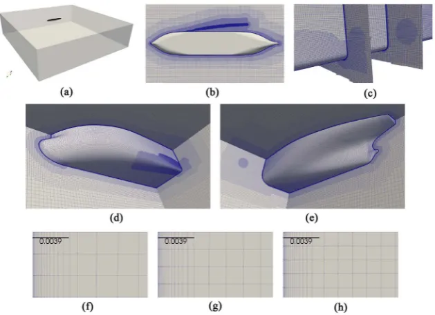
Compuational domain: mesh and boundary conditions Figure 6(a) represents the computational domain which extends for 6Loa in x- and y-direction and

for 1.5Loa in z-direction. Three meshes are created to investigate the

discretisa-tion error, a coarse, a medium and a fine one. The OpenFOAM meshing tool snappy HexMesh (version 1806) is used therefore: Starting from a homogeneous and isotropic block mesh, the cells in the vicinity of the hull are refined and snapped to the surface. Finally, cell layers are introduced on the hull surface for the resolution of the boundary layer flow. See Figure 6 for different views of the mesh and Table 4 for general and detailed information.

The different meshes coarse, medium and fine are created by refining the background block mesh with a factor of exactly 1.25. The cell count along the domain edges in z-direction changes from 16 (coarse mesh) to 20 (medium) to 25 (fine) and in x- and y-direction with the same ratio. As the body mesh and the refinement regions are based on the block mesh, the cell size ratio is also 1.25.

[image:10.595.217.532.430.658.2]

(11)

[image:11.595.210.540.113.386.2]

DOI: 10.4236/ojfd.2019.94020 313 Open Journal of Fluid Dynamics Table 4. Parameters of the mesh. Absolute layer thickness in [mm] refers to layers with cell level 6; the values are set in relation to the cell size of level 6 which covers most of the hull and the near wake.

Coarse Medium Fine Total cell count 6.4 M 10.5 M 17.5 M

Mesh refinement 1 1.25 1.252

Cell size level 0 150 mm 120 mm 96 mm Cell size level 6 2.34 mm 1.88 mm 1.50 mm Cell size level 7 1.17 mm 0.94 mm 0.75 mm

Layer count 19 19 19

Layer extrusion ratio 1.2 1.2 1.2 1st layer thickness 3.15e-2 mm 2.52e-2 mm 2.02e-2 mm

/level 6 1.34% 1.34% 1.34%

Last layer thickness 0.84 mm 0.67 mm 0.54 mm

/level 6 36% 36% 36%

Total layer thickness 4.5 mm 3.9 mm 3.1 mm

/level 6 210% 210% 210%

/1st layer th. 155 155 155

Faces non-ortho >70˚ 13 35 56

The mesh structure The block mesh is considered level 0, the cells at the hull and around the FSV are isotropically refined six times (up to level 6 respectively) and up to level 7 at four distinct zones (see also Figure 7(a): blue-level 6, red-level 7):

 bow: high velocity magnitude due to the flow around the corner;

 _{stern: small geometry features to capture by the mesh;}

 _{FSV initial separation (until}

x L

_pp

≈

0.33

): high mesh density to resolve

ini-tial vortex formation and roll up of free shear layer;

 FSV core (until

x L

_pp

≈

0.73

): vortex core where high flow gradients occur.

Following the vortex core line of a preliminary result on the medium mesh the cells are refined within a certain distance around it.

(12)

For the coarse and medium mesh the layer coverage on the hull is 100%, for the medium mesh there is a tiny part (below 0.3% of the hull surface) where no or less than 19 layers are extruded by the mesh algorithm. This part is located near the forward shoulder and the waterline at the windward side (starboard). As this is located close the stagnation point where the flow velocity is small, no serious influence on the result is observed.

According to [23] the semi viscous zone Y+<30 of the boundary layer should

be discretised for low-Re RANS boundary conditions with five to ten cells. As-suming Y+ =1 the expansion factor 1.2 leads to nearly eight layer cells within

the semi viscous zone. Comparing to Figure 7 the boundary layer flow is prop-erly resolved, where the coarse mesh has comparatively few cells but still around five.

At the hull the only no-slip boundary condition is preset, the imaginary wa-tersurface is modelled with a slip (zero-gradient) condition, both inlet patches with a velocity inlet setting the velocity magnitude to U∞ =25 m s and the

in-flow angle to 30˚ and the outlet is modelled with a pressure outlet condition (with undisturbed static pressure p∞ =0).

5. Results

First, the near wall resolution and the resolved turbulent energy are analysed. Afterwards, the investigation deals with the vortex structures, local flow effects, the development at the vortex core line and the wall shear. Most results are ob-tained with CFD, only the vortex core flow also compared to PIV data.

[image:12.595.211.536.479.565.2]

CFD verification The flow near the ship hull is computed in RANS mode down to the wall, so without wall functions. As required the dimensionless wall distance is near unity, see Table 5. The decrease of the average value (from coarse

Figure 7. Near wall mesh resolution, dimensionless wall distance Y+ based on time-

averaged flow. Small Y+ values correspond to small cell sizes on the hull. (a) Cell level

at the hull, blue-level 6, red-level 7; (b) Coarse; (c) Medium; (d) Fine.

Table 5. Dimensionless wall distance Y+ for all meshes based on the time-averaged

flow: minimum, maximum and average values.

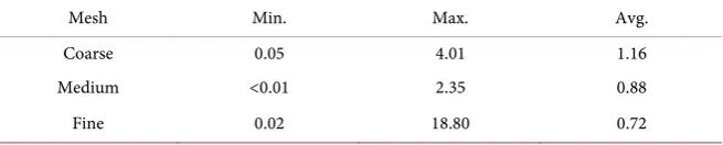
Mesh Min. Max. Avg.

Coarse 0.05 4.01 1.16

Medium <0.01 2.35 0.88

[image:12.595.211.539.659.725.2]

(13)

to fine) arises due to the refinement of the first cell. The high maximum value for the fine mesh originates from the missing layer extrusion mentioned above. Analysing the local flow the impact is considered negligible.

The wall distance and the wall near flow are presented in Figure 7. The small

Y+ values downstream of the port shoulder of the hull originate from the mesh

refinement in this region which provides a fine resolution of the initial FSV re-spectively. Considering the colour legend the wall distance is predominantly be-low unity for the medium and fine mesh. Possible explanations for higher values on the coarse mesh are the larger first layer cell and unsteady oscillations which lead to high velocities. This corresponds to the high amount of resolved TKE (refer Figure 9(g)) and the vortex pattern of the instantaneous flow (visualised with Q-isolines in Figure 10(a) and Figure 10(d)).

Considering the hybrid RANS-LES approach, the RANS-LES interface and the amount of resolved TKE is analysed in the following. Figure 9(d), Figure 9(e) and Figure 9(f) show that RANS is active near the hull and both the separated free shear layer and the FSV are resolved with LES. The resolved TKE near the shear layer which separates at the bilge corner develops quickly as can be seen in subfigures Figure 9(g), Figure 9(h) and Figure 9(i).

Furthermore the proper resolution of hybrid RANS-LES or LES approaches can be verified with the relation of resolved TKE to total TKE

1 2 1 2

i i

res tot

i i mod

u u

k k

u u k

′ ′ =

′ ′ + (2)

using the trace of the reynolds stress tensor 1

2 u ui′ ′i and TKE from the subgrid

model kmod. As originally proposed in [24], at least 80% of the total TKE should

be resolved, kres ktot >80%. Considering Figure 9(g), Figure 9(h) and Figure

9(i) the level is above 90% inside the tip vortex core and the free shear layer that rolls up. In the surrounding refined region the level is still above 80%. Following the bulk of turbulent energy can be considered resolved. The large level of re-solved TKE on the coarse mesh corresponds to the velocity fluctuations with high amplitude observed. A possible explanation are numerical instabilities that originate from the mesh resolution as these effects are not present on the me-dium and fine mesh.

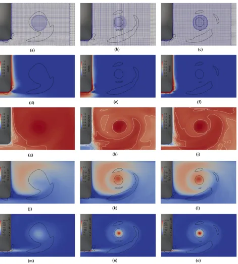
Flow analysis Within the following section different aspects of the flow are analysed starting with the vortical structures in the vicinity of the FSV followed by a local analysis at a plane, the flow at the vortex core line and the limiting streamlines.

(14)

[image:14.595.215.533.73.287.2]

DOI: 10.4236/ojfd.2019.94020 316 Open Journal of Fluid Dynamics Figure 8. Instantaneous (left column) and time-averaged (right column) vortex structures

represented by 2 2

100

pp

QL U∞= for the coarse (top), medium (centre) and fine (bottom) mesh. Downstream of the refinement the isosurfaces are clipped. Isosurfaces coloured by normalized helicity, blue represents −1, red +1. (a) Medium, instantaneous and mesh; (b) Colour legend; (c) Coarse, instantaneous; (d) Coarse, time-averaged; (e) Medium, instan-taneous; (f) Medium, time-averaged; (g) Fine, instaninstan-taneous; (h) Fine, time-averaged.

resolution becomes visible as the size of the FSV isosurface decreases from coarse to medium. On the medium and the fine mesh the difference is small; this corresponds to the grid convergence of the results discussed below.

Plenty vortices of different size are visible in the instantaneous flow field. The pattern on the medium and fine mesh is similar and the vortices are restricted to the refined mesh zone. On the coarse mesh, larger scales occur. In general the instantaneous vortex pattern consists of circular structures surrounding the FSV, these patterns represent the separated free shear layer that rolls up and induces velocities onto the FSV. This observation was also mentioned in [12].

Local flow analysis In the following the flow at plane perpendicular to the vortex axis will be analysed, see Figure 9 for the time-averaged flow. The plane is located near A-A in Figure 1. The black isolines indicate the vortex core and the free shear layer, its value is lower than in Figure 8 to get more information on the free shear layer. First, the mesh shows the circular refinement for the vortex core (level 7). On the coarse mesh the vortex core is significantly larger than on both other meshes and the core is bigger than the refinement. Following, the RANS-LES blending and the resolved TKE have been analysed above con-cluding that both free shear layer and FSV are properly resolved with LES.

(15)

[image:15.595.65.537.67.592.2]

DOI: 10.4236/ojfd.2019.94020 317 Open Journal of Fluid Dynamics Figure 9. Different flow fields at x L_pp=0.6 (near A-A in Figure 1(a)) based on time-averaged fields for the three meshes: left-coarse, centre-medium, right-fine. Black isolines represent 2 2

22.6

pp

QL U_∞= , white isolines represent TKE resolved by total in

steps of 0.1. (a)-(c) mesh; (d)-(f) blending between LES and RANS; (g)-(i) resolved TKE to total TKE; (j)-(l) axial velocity; (m)-(o) axial vorticity.

(16)

[image:16.595.62.540.470.685.2]

On the coarse mesh, two effects occur: the lower resolution is a possible ex-planation for the weaker vortex (increased numerical diffusion) but still the ve-locity oscillations lead to a high TKE level. So there are many flow instabilities or fluctuations which seem to have a numerical origin, at least they do not contri-bute to a coherent vortex structure. For example, as seen in Figure 9(g), the level of resolved to total TKE is higher than on the finer meshes an does not represent the vortex pattern.

Figure 10 presents the velocity and vorticity on the plane for the instantane-ous flow at the last simulated time step. The numerinstantane-ous vortical structures that can be seen in Figure 8 are represented by the black isolines (here, the isovalue is different). As stated above, there are more structures on the coarse mesh than on the others, especially outside of the region where the FSV rolls up. On the coarse mesh, high velocity areas occur at the vortex centre and near the hull. On the medium and the fine mesh there are several regions with a velocity overshoot near the vortex centre.

In the vorticity field, the current pattern of the free shear layer can be deter-mined. It consists of zones with different axial vorticity which represents the un-steady nature of the flow separation. The local maximum at the vortex centre is clearly visible; most of the vorticity is concentrated there.

Although it is a snapshot of the unsteady wake flow, the vortex core of the FSV can be determined. This fact can be used to analysed a possible wandering motion of the FSV: Wandering is expected to occur at very low frequencies compared to turbulent fluctuations [3]. As the coherent vortex can be identified already at the instantaneous flow field (or a short time-averaged field), its posi-tion can be tracked in time. Hence, a possible wandering moposi-tion could be ana-lysed.

Figure 10. Different flow fields at x Lpp=0.6 (near A-A in Figure 1(a)) based on instantaneous fields for the three meshes: left-coarse, centre-medium, right-fine. Black isolines represent 2 2

22.6

pp

(17)

Vortex core properties The algorithm to extract the centre of the FSV is based on the local alignment of the velocity and the vorticity vector (the normalized helicity is the cosine between both vectors), as the velocity is parallel to the vor-ticity at the vortex centre. It was proposed by Levy and colleagues in [25] and the implementation was obtained from [26]. Within postprocessing the algorithm is used inside the paraview framework to extract the FSV core line on each mesh separately for the time-averaged flow.

[image:17.595.213.534.247.657.2]

The axial velocity, vorticity, the pressure coefficient and the resolved TKE at the vortex centre as well as its position are shown in Figure 11. First, the overall development of the curves is described, afterwards the curves for the medium and fine mesh are analysed in detail.

(18)

Considering the pressure coefficient it is necessary to mention that the undis-turbed static pressure p∞ is zero, so the numerator becomes p−p∞ = p. All

subfigures show similar results for the medium and fine mesh, but the vortex on the coarse mesh is significantly weaker (smaller vorticity and higher pressure). Considering that the cell size changes with a factor of 1.25 from mesh to mesh, the time-averaged flow shows grid convergence because the change from coarse to medium is large and from medium to fine is about an order smaller. As the resolution of the coarse mesh is considered not sufficient, the vortex core prop-erties are not analysed in the following.

At the initial vortex evolution the pressure reduction and the velocity over-shoot develop on a short distance compared to the decay further downstream. Near

x L

_pp

=

0.3

the extremal value is (nearly) reached and both the velocity

and the pressure decrease at a similar rate to approximately 90% of their extrem-al vextrem-alues at

x L

_pp

=

0.73

. The vorticity shows a small peak near

x L

_pp

=

0.3

with a sudden decrease by about 10%, further downstream the vorticity decreas-es linearly to about 50% of the extremal value. Near

x L

_pp

=

0.33

the mesh

coarsens, the refinement box around the free shear layer and at the hull where the FSV separates ends, see Figure 6(c) and Figure 7. This is an explanation for the bump in the velocity and pressure curves as well as for the sudden decrease of the vorticity. Besides, this presents a motivation to refine the mesh around the free layer which seems to have a large influence on the vortex core vorticity.

The resolved TKE is approximately two orders of magnitude larger than the modelled part, this corresponds to the observations in Figure 9(g), Figure 9(h) and Figure 9(i). After rising to approximately 0.05 the resolved TKE increases little further downstream. Following, the resolved turbulent energy keeps at a certain level when the FSV rolls up.

Comparison of the vortex core flow to PIV data For the experimental re-sults, the vortex core line is extracted by local extrema of the axial vorticity. It is assumed that the influence of the different vortex core line algorithms is negligi-ble as usually the vorticity has a local extremum at the vortex centre for a cohe-rent structure. At least the difference in the algorithms cannot explain the dis-crepancy in the vorticity level.

The shaded region in Figure 11 represents the bandwidth of the experimental results. The solid lines represent the minimum and maximum value of the mean velocity, vorticity and position resulting from the data reduction. Considering the core velocity it reaches the velocity overshoot further downstream and its value is about 15% smaller than the one of the CFD result. A nearly constant level of vorticity of about 200 is predicted by the experiments. The initial value predicted by CFD is much higher but decreases as the FSV trails downstream. Referring to the vortex centre position, the initial FSV is attracted by the hull surface at small y values. Further downstream is follows a line.

(19)

may be induced. During the postprocessing of the PIV data the flow field is av-eraged on a fixed grid, see Equation (1). Vortex wandering may lead to a smooth-ing of the high velocity gradients in the vortex core which in turn would lead to a reduced vorticity level.

Limiting streamlines The limiting streamlines shown in Figure 12 indicate separation and reattachment lines. Proceeding from the bow downstream the Fore-body Bilge Vortex (FBV, see Figure 1) is located at the leeward shoulder where the streamlines bend around the FBV. The free shear layer that rolls up into the FSV originates from the separation on the leeward bilge, see e.g. [4] for experimental results or [12]. As the surface curvature is high at the bilge the se-paration point is preset and captured well by the flow simulation. On the wind-ward bilge the flow separates and forms the Aft-body Side Vortex (ASV) which is located between the separation and reattachment lines. Between the aft shoul-der and the propeller hub the ASV separates from the hull’s bottom.

6. Conclusions

[image:19.595.262.485.513.682.2]

The current results provide a basis for future research on the resolution of co-herent vortices with proper RANS models (e.g. with curvature correction) or scale resolving simulations. The hybrid RANS-LES approach based on the k-ω-SST-IDDES model seems to be well suited for the prediction of the FSV at 30˚ drift angle as the LES region around the FSV is properly resolved and the time-averaged flow at the vortex core line shows grid convergence. A proof for the proper resolution inside the LES region is the high value of resolved to total TKE which is mostly higher than 80% and near unity inside vortex core and free shear layer. Grid convergence can be assumed as the time-averaged velocity, vor-ticity, pressure and the resolved TKE at the vortex centre as well as its location change very little from the medium to the fine mesh compared to a large differ-ence from the coarse to the medium mesh. Besides, the instantaneous vortical

(20)

structures on both finer meshes have a similar pattern.

Considering the grid study, the results on the coarse mesh differ significantly from the ones on both finer meshes. Taking into account high-velocity fluctua-tions whose origin seems to be a numerical issue, the coarse mesh may be too coarse to properly resolve the flow. Hence, the following conclusions on the flow are referred to the medium and fine mesh.

The vortex pattern of the time-averaged and instantaneous flow is quite dif-ferent: For the first a coherent smooth vortex tube exists and for the latter there are many small vortical structures wrapping around the FSV. Even for the in-stantaneous flow the nearly circular shape of the FSV core was observed for one time step. This observation supports the dominant nature of a trailing vortex.

The comparison of the PIV and CFD results for the vortex core shows that the position coincides well, the velocity overshoot is about 15% higher for CFD and the vorticity is initially about 100% higher but decreases to the constant experi-mental value. The reason for the deviation is not certain; a possible explanation is the smoothing of the experimental data due to the analysis on a fixed grid that does not consider a possible wandering motion of the FSV in the wind tunnel.

Outlook Several aspects will be analysed in the future considering validation, different modelling and numerical approaches and a comparison to other flows with coherent trailing vortices:

 As the coarse mesh shows convergence issues and high-velocity fluctuations without proper physical explanation, meshes with a resolution between the coarse and medium ones should be investigated.

 The promising results of the medium and fine mesh lead to the question whether the approach is applicable to smaller drift angles that occur in the everyday operation of ships. A first test case would be the drift angle 12˚.

 As the free shear layer rolls up into the FSV it may induce axial velocity to the vortex core. This can be further investigated by refining the the region where the shear layer is located.

 _{After the analysis of the initial separation and the separate development of}

the FSV it would be of interest to analyse its interaction further downstream inside the vortex wake, see Figure 1. The highly turbulent wake flow may contain distinct peak frequencies that match some of the hull forces. To achieve a proper resolution of the ASV that develops at least partly inside the boundary layer flow and therewith the RANS zone requires special treatment: a possible approach is the consideration of curvature correction for the RANS model.

 Another point considering the modelling refers to the comparison of differ-ent kinds of turbulence models. Possible models need to consider the strong curvature inside the vortex core, e.g. with curvature correction or like in EARSM framework. These RANS models offer a huge gain in computational efficiency and the question is how accurate the vortex flow can be predicted.

(21)

occurs in EFD and/or CFD and quantified. Besides, the measured data needs to be corrected for the wandering motion. A possible initial approach can be based on the observation that the vortex centre and the vortex core pattern seem to be present even for the instantaneous flow. Hence, the wandering motion could be tracked. This needs to be considered within future experi-mental and numerical investigations.

Acknowledgements

This research was partially sponsored by the Office of Naval Research Global under Grant N62909-18-1-2080 under the administration of Drs Salahuddin Ahmed and Wei-Min Lin. The authors would like to express their thanks for the support. Besides, the authors would like to thank their colleagues Klaus Wieczo-rek, Dr. Volker Müller and Jörg Voigt for their work related to the experiments.

Disclaimer

Any opinions, findings, and conclusions or recommendations expressed in this material are those of the authors and do not necessarily reflect the views of the Office of Naval Research.

Conflicts of Interest

The authors declare no conflicts of interest regarding the publication of this pa-per.

References

[1] Gritskevich, M.S., Garbaruk, A.V., Schutze, J. and Menter, F.R. (2012) Development of DDES and IDDES Formulations for the k-ω Shear Stress Transport Model. Flow,

Turbulence and Combustion, 88, 431-449.

https://doi.org/10.1007/s10494-011-9378-4

[2] Chow, J.S., Zilliac, G.G. and Bradshaw, P. (1997) Mean and Turbulence Measure-ments in the Near Field of a Wingtip Vortex. AIAA Journal, 35, 1561-1567.

https://doi.org/10.2514/2.1

[3] Devenport, W.J., Rife, M.C., Liapis, S.I. and Follin, G.J. (1996) The Structure and Development of a Wing-Tip Vortex. Journal of Fluid Mechanics, 312, 67-106.

https://doi.org/10.1017/S0022112096001929

[4] Abdel-Maksoud, M., Muller, V., Xing, T., Toxopeus, S., Stern, F., Petterson, K., et al. (2015) Experimental and Numerical Investigations on Flow Characteristics of the Kvlcc2 at 30 Drift Angle. 5th World Maritime Technology Conference, Rhode Isl-and, 3-7 November 2015, 139-164.

[5] Larsson, L., Stern, F. and Bertram, V. (2003) Benchmarking of Computational Fluid Dynamics for Ship Flows: The Gothenburg 2000 Workshop. Journal of Ship Re-search, 47, 63-81.

[6] Larsson, L., Stern, F. and Visonneau, M. (2010) Gothenburg 2010, a Workshop on Numerical Ship Hydrodynamics. Technical Report, Chalmers University of Tech-nology, Göteborg.

(22)

Re-DOI: 10.4236/ojfd.2019.94020 324 Open Journal of Fluid Dynamics sults of the Gothenburg 2010 Workshop. In: Marine 2011, IV International Confe-rence on Computational Methods in Marine Engineering, Springer, Berlin, 237-259.

https://doi.org/10.1007/978-94-007-6143-8_14

[8] Larsson, L., Stern, F. and Visonneau, M. (2013) Numerical Ship Hydrodynamics: An Assessment of the Gothenburg 2010 Workshop. Springer, Berlin.

https://doi.org/10.1007/978-94-007-7189-5

[9] Hino, T. (2005) CFD Workshop Tokyo 2005. National Maritime Research Institute, Tokyo.

[10] Stern, F. (2009) Lessons Learnt from the Workshop on Verification and Validation of Ship Maneuvering Simulation Methods SIMMAN 2008. Proceedings of Interna-tional Conference on Marine Simulation and Ship Maneuverability, Copenhagen, 14-16 April 2008.

[11] Stern, F. and Agdrup, K. (2008) SIMMAN 2008 Workshop on Verification and Va-lidation of Ship Maneuvering Simulation Methods. Draft Workshop Proceedings. [12] Fureby, C., Toxopeus, S., Johansson, M., Tormalm, M. and Petterson, K. (2016) A

Computational Study of the Flow around the KVLCC2 Model Hull at Straight Ahead Conditions and at Drift. Ocean Engineering, 118, 1-16.

https://doi.org/10.1016/j.oceaneng.2016.03.029

[13] Xing, T., Bhushan, S. and Stern, F. (2012) Vortical and Turbulent Structures for KVLCC2 at Drift Angle 0, 12, and 30 Degrees. Ocean Engineering, 55, 23-43.

https://doi.org/10.1016/j.oceaneng.2012.07.026

[14] Xing, T., Shao, J. and Stern, F. (2007) BKW-RS-DES of Unsteady Vortical Flow for KVLCC2 at Large Drift Angles. Proceedings of the 9th International Conference on Numerical Ship Hydrodynamics, Ann Arbor, August 2007, 5-8.

[15] Ismail, F., Carrica, P.M., Xing, T. and Stern, F. (2010) Evaluation of Linear and Nonlinear Convection Schemes on Multidimensional Non-Orthogonal Grids with Applications to KVLCC2 Tanker. International Journal for Numerical Methods in Fluids, 64, 850-886. https://doi.org/10.1002/fld.2174

[16] Van, S.H., Yim, G.T., Kim, W.J. and Kim, D.H. (1997) Measurement of Flows around 3600 TEU Container Ship Model. Proceedings of Annual Autumn Meet-ings, Seoul, 300-304.

[17] Menter, F., Kuntz, M. and Langtry, R. (2003) Ten Years of Industrial Experience with the SST Turbulence Model. Turbulence, Heat and Mass Transfer, 4, 625-632. [18] Shevchuk, I. (2016) Study of Unsteady Hydrodynamic Eﬀects in the Ship Stern Area

under Shallow Water Conditions. PhD Thesis, University of Rostock, Rostock. [19] Weller, H.G., Tabor, G., Jasak, H. and Fureby, C. (1998) A Tensorial Approach to

Computational Continuum Mechanics Using Object-Oriented Techniques. Com-puters in Physics, 12, 620-631. https://doi.org/10.1063/1.168744

[20] Issa, R.I. (1986) Solution of the Implicitly Discretised Fluid Flow Equations by Op-erator-Splitting. Journal of Computational Physics, 62, 40-65.

https://doi.org/10.1016/0021-9991(86)90099-9

[21] Vuorinen, V., Keskinen, J.-P., Duwig, C. and Boersma, B. (2014) On the Implemen-tation of Low-Dissipative Runge-Kutta Projection Methods for Time Dependent Flows Using OpenFOAM. Computers & Fluids, 93, 153-163.

https://doi.org/10.1016/j.compfluid.2014.01.026

[22] Strelets, M. (2001) Detached Eddy Simulation of Massively Separated Flows. 39th Aerospace Sciences Meeting and Exhibit, Reno, 8-11 January 2001, 879.

(23)

DOI: 10.4236/ojfd.2019.94020 325 Open Journal of Fluid Dynamics [23] Rung, T. (2002) Statistische Turbulenzmodellierung. Lecture Notes.

[24] Pope, S.B. (2000) Turbulent Flows. Cambridge University Press, Cambridge.

https://doi.org/10.1017/CBO9780511840531

[25] Degani, D., Seginer, A. and Levy, Y. (1990) Graphical Visualization of Vortical Flows by Means of Helicity. AIAA Journal, 28, 1347-1352.

https://doi.org/10.2514/3.25224