Galaxy And Mass Assembly (GAMA): M⋆ Re relations of z = 0 bulges, discs and spheroids

MNRAS462,1470–1500 (2016) doi:10.1093/mnras/stw1495 Advance Access publication 2016 July 6

Galaxy And Mass Assembly (GAMA):

M

–

R

e

relations of

z

=

0 bulges,

discs and spheroids

Rebecca Lange,

Amanda J. Moffett,

Simon P. Driver,

Aaron S. G. Robotham,

Claudia del P. Lagos,

Lee S. Kelvin,

Christopher Conselice,

Berta Margalef-Bentabol,

Mehmet Alpaslan,

Ivan Baldry,

Joss Bland-Hawthorn,

Malcolm Bremer,

Sarah Brough,

Michelle Cluver,

Matthew Colless,

Luke J. M. Davies,

Boris H¨außler,

Benne W. Holwerda,

Andrew M. Hopkins,

Prajwal R. Kafle,

Rebecca Kennedy,

Jochen Liske,

Steven Phillipps,

Cristina C. Popescu,

Edward N. Taylor,

Richard Tuffs,

Eelco van Kampen

and Angus H. Wright

Affiliations are listed at the end of the paper

Accepted 2016 June 20. Received 2016 May 25; in original form 2016 February 14

A B S T R A C T

We perform automated bulge+disc decomposition on a sample of ∼7500 galaxies from the Galaxy And Mass Assembly (GAMA) survey in the redshift range of 0.002< z <0.06 using Structural Investigation of Galaxies via Model Analysis, a wrapper aroundGALFIT3. To

achieve robust profile measurements, we use a novel approach of repeatedly fitting the galaxies, varying the input parameters to sample a large fraction of the input parameter space. Using this method, we reduce the catastrophic failure rate significantly and verify the confidence in the fit independently ofχ2_{. Additionally, using the median of the final fitting values and}

the 16th and 84th percentile produces more realistic error estimates than those provided by

GALFIT, which are known to be underestimated. We use the results of our decompositions to

analyse the stellar mass – half-light radius relations of bulges, discs and spheroids. We further investigate the association of components with a parent disc or elliptical relation to provide definitez = 0 disc and spheroid M–Re relations. We conclude by comparing our local

disc and spheroidM–Reto simulated data fromEAGLEand high-redshift data from Cosmic

Assembly Near-infrared Deep Extragalactic Legacy Survey-Ultra Deep Survey. We show the potential of using theM–Rerelation to study galaxy evolution in both cases but caution that

for a fair comparison, all data sets need to be processed and analysed in the same manner.

Key words: galaxies: elliptical and lenticular, cD – galaxies: formation – galaxies: fundamen-tal parameters – galaxies: spiral – galaxies: statistics.

1 I N T R O D U C T I O N

At the fundamental level, galaxies are multicomponent systems

(see for example Buta et al.2010), consisting of at least a spheroid

and/or disc. This is most obvious in the S´ersic index–colour plane where the single-component Sd and elliptical galaxies occupy dis-tinct peaks with composite galaxies (S0abc) scattered between and

around these peaks (see e.g. Driver et al. 2006; Cameron et al.

2009; Kelvin et al.2012; Lange et al.2015). These components

_{E-mail:rebecca.lange@icrar.org(RL);simon.driver@icrar.org(SPD)}

have very different characteristics with spheroids typically having a featureless appearance and being pressure-supported. Discs, on the other hand, have features such as spiral arms and are rotationally supported. Furthermore, bulges are made up of redder stars with

moderate to high metallicities and a highα-element abundance,

while discs are made of younger, bluer stars with lower metal-licities and typically are dust- and gas-rich. Spheroids are older, showing little to no star formation and are typically dust- and

gas-depleted (see for example the review by Roberts & Haynes1994).

The simplest explanation for these stark differences is that spheroids and discs form via two distinct mechanisms over two distinct eras

(Cook, Lapi & Granato2009; Driver et al.2013), i.e. a dynamically

at University of St Andrews on October 11, 2016

http://mnras.oxfordjournals.org/

‘hot mode’ (spheroid formation) and ‘cold mode’ (disc formation) evolution.

Traditionally, the relative prominence of a bulge component is

taken into account when classifying galaxies on to theHubble

se-quence (see Hubble1926, and later revisions by e.g. van den Bergh

1976; Kormendy & Bender2012), however, studying global

prop-erties of galaxies byHubbletype could be misleading. For example,

numerous evolution mechanisms have been proposed to explain the

morphological diversity seen atz =0, such as a (initial) major

dissipative event, gas accretion, adiabatic contraction, major and

minor mergers and secular processes (see e.g. Hopkins et al.2010;

Trujillo, Ferreras & Rosa 2011; L’Huillier, Combes & Semelin

2012; Cheung et al.2013; Sachdeva et al. 2015). Each of these

processes potentially acts to modify the prominence of the bulge, disc or other components. This indicates that galaxy components likely follow distinct formation pathways and structure effectively encodes the formation history. Therefore, to study galaxy evolution,

bulge+disc decomposition is critical.

While the number of studies of large samples which employ

bulge+disc decomposition to explore the nature of galaxies and

their components is growing, the analysis is challenging (see e.g.

Allen et al.2006; Gadotti2009; Simard et al.2011; Bruce et al.

2012,2014; Lang et al.2014; Tasca et al.2014; Meert, Vikram &

Bernardi2015; Salo et al.2015). This is because multicomponent

fitting is notoriously difficult, especially when trying to automate it for large samples. Nevertheless, a number of publicly available

codes have now been created to allow bulge+disc decomposition,

such asGIM2D(Simard1998),BUDDA(de Souza, Gadotti & dos Anjos

2004),GALFIT3 (Peng et al.2010) andIMFIT(Erwin2015). Each code

has advantages and disadvantages (see Erwin2015, for example,

for further discussion), here we elect to useGALFIT3 because of its

ability to manage nearby objects, its computational reliability, and its speed.

Many studies that fit two-component S´ersic light profiles restrict

the S´ersic index ton=1 for the disc and in some cases, n= 4

for the bulge (e.g. Simard et al.2011; Bruce et al.2012;

Lack-ner & Gunn2012; Meert et al.2015). This reduces the number

of free parameters and ensures the fitting process is more robust but it restricts the possible interpretations of the fitting outcomes, e.g. classical and pseudo-bulges cannot be differentiated this way. A number of studies now show that the S´ersic index of discs and spheroids (be they pure or component) vary smoothly with mass and luminosity or due to dust or galaxy type (see e.g. Graham &

Guzman2003; Gadotti 2009; Kelvin et al.2012; Graham 2013;

Pastrav et al.2013a,b). Hence, studies where the S´ersic index of

the bulge or disc components are fixed may be overly restrictive. Furthermore, to correctly trace a galaxy’s formation history, a full decomposition of all of its components would be ideal (e.g. the

Spitzer Survey of Stellar Structure in Galaxies, S4_{G; Salo et al.}

2015). However, this is only viable for very nearby galaxies where

all the components can be clearly resolved and hence for

rela-tively small samples (S4_{G is the largest study to date extending}

to 2352 galaxies for which a number have been fit with more than two components). To compare galaxies at different epochs going beyond a simple bulge and disc decomposition is difficult

(Gadotti2008). There are two reasons, however, why two

compo-nents might be sufficient, (i) the majority of stellar mass resides in the bulge and disc components for most galaxies, and (ii) some components may simply represent minor perturbations to the un-derlying disc (e.g. bars, pseudo-bulges). Such perturbations should arguably be considered secondary rather than primary evolutionary markers.

Here we adopt the stance that bulge and disc components arise from two primary formation pathways (i.e. hot and cold mode evo-lution, respectively), and that additional components form in sec-ondary formation pathways (i.e. tidal interactions, disc instabilities and perturbations). The likely primary pathways are: monolithic collapse followed by major mergers, which can produce elliptical galaxies by destroying and rearranging any structure previously present in a galaxy, resulting in a smooth light profile (Toomre

1977); and minor mergers and continued gas inflow, which can

form or re-grow a disc around a pre-existing spheroid, resulting in a galaxy with two distinct components (see e.g. Steinmetz &

Navarro2002; Kannappan, Guie & Baker2009; Wei et al.2010).

A key question worth asking is whether two generic components (spheroids and discs) really can explain the diversity seen, i.e. how many fundamental building blocks and structures are required to adequately reproduce the observed galaxy population? As most of the stellar mass is contained within the bulge and disc, how important are tertiary features like bars? Furthermore, how many different physical origins do the various spheroids and discs have? Are elliptical galaxies simply naked bulges and are bulges related

to high-redshift compact galaxies (e.g. Berg et al.2014; Graham,

Dullo & Savorgnan2015)? Are the discs of early types, late types

and irregulars indistinguishable?

We believe that the stellar mass – half-light size (hereafter

M–Re) relation is a key scaling relation allowing us to address

these questions for the following reasons.

(i) The size of a galaxy is related to its specific angular momen-tum making the mass and size of a galaxy fundamental observables

of conserved quantities (e.g. Romanowsky & Fall2012).

(ii) The simple assumption that angular momentum is conserved during the initial collapse of the dark matter halo links the angular momentum and mass of a galaxy with its dark matter halo (Fall &

Efstathiou1980; Dalcanton, Spergel & Summers1997; Mo, Mao

& White1998).

(iii) Hydrodynamical simulations now produce galaxies with re-alistic sizes and direct comparisons (at different epochs) are possi-ble to study formation and evolution histories of galaxies (see for example, the Evolution and Assembly of Galaxies and their

Envi-ronments simulation suite,EAGLE; Crain et al.2015; Schaye et al.

2015).

(iv) We can empirically measure and trace the masses and sizes of galaxies and their components over a range of redshifts and in

different environments [e.g. withHubble Space Telescope(HST) as

well as high-redshift ground-based surveys and soon withEuclid

and Wide-Field Infrared Survey Telescope (WFIRST)].

TheM–Rerelation therefore represents the next critical

diag-nostic for galaxy evolution studies beyond simple mass functions

(see e.g. Bouwens et al.2004; van der Wel et al.2014; Holwerda

et al.2015; Shibuya, Ouchi & Harikane2015), enabling us to trace

angular momentum build-up and the emergence of the component nature of galaxies while connecting observations to simulations.

Recent studies comparing theM–Rerelation of low and high

redshift are already yielding interesting results. For example, at high redshift, galaxies might look disc-like or elliptical/spheroidal, but their physical properties are unlike any discs or ellipticals in the local

Universe (see e.g. Bruce et al.2012; Buitrago et al.2013; Mortlock

et al.2013). Galaxies at high redshifts are typically more irregular

with thick slab-like disc structures and clumpy star-forming regions

(Wisnioski et al.2012). In addition, they can be very compact but

massive. In some cases, at redshift∼2, they are a factor of up to

6 times smaller in size than galaxies of the same mass today (Daddi

at University of St Andrews on October 11, 2016

http://mnras.oxfordjournals.org/

1472

R. Lange et al.

et al.2005; Trujillo et al.2007; Buitrago et al.2008; van Dokkum

et al.2008,2010; Weinzirl et al.2011).

In this paper, we aim to provide a reliable low-redshift benchmark

of theM–Rerelation for bulges, discs and spheroids. The bulge

+disc decomposition sample is derived from a set of galaxies for

which detailed morphological information is available (see Moffett

et al.2016). Section 2 describes the data and sample selection,

Sec-tions 3 and 4 describe the set up of our bulge+disc decomposition

catalogue and component mass estimates. In Section 5, we present

theM–Rerelations for bulges, spheroidal and disc galaxies and

discuss the association of components with their possible parent

populations. We then compare our distributions to theEAGLE

sim-ulation in Section 6 followed by a comparison of our low-redshift

M–Re relation with recent high-redshift data from Ultra Deep

Survey (UDS) region within the Cosmic Assembly Near-infrared

Deep Extragalactic Legacy Survey (CANDELS; Grogin et al.2011;

Koekemoer et al.2011) in Section 7. Finally, in Section 8, we present

our summary and conclusions.

Throughout this paper, we use data derived from the Galaxy

And Mass Assembly (GAMA) survey (Driver et al.2011,2016;

Liske et al.2015) with stellar masses derived from Taylor et al.

(2011), sizes derived from S´ersic profile fitting using Structural

Investigation of Galaxies via Model Analysis (SIGMA; Kelvin et al.

2012), and for a cosmology given by:cold dark matter (CDM)

universe withm=0.3,=0.7,H0=70 km s−1Mpc−1.

2 DATA

The GAMA survey is an optical spectroscopic and multiwavelength

imaging survey of∼300 000 galaxies, combining the data of several

ground- and space-based telescopes (Driver et al.2011,2016). It is

an intermediate survey in respect to depth and survey area (Baldry

et al.2010) and thus fits in between low-redshift, wide-field surveys

such as SDSS (York et al.2000) or 2dFGRS (Colless et al.2003)

and narrow deep field surveys like zCOSMOS (see Lilly et al.2007

and Davies et al.2015) or DEEP-2 (Davis et al.2003).

In this paper, we use data from the GAMA II (Liske et al.2015)

equatorial regions, which are centred on 9h (G09), 12h (G12) and

14.5h (G15). The three regions are 12×5 deg2_{in extent and have}

anrband Petrosian magnitude limit of r<19.8 mag. The

spec-troscopic target selection is derived from SDSS DR 7 (Abazajian

et al.2009; see Baldry et al.2010for details) input catalogue and

we reach a spectroscopic completeness of≥98 per cent for the main

survey targets. The redshifts (Baldry et al.2014; Liske et al.2015)

are based on spectra taken with the AAOmega spectrograph at the

3.9m Anglo–Australian Telescope (Hopkins et al.2013) located at

Siding Spring Observatory. The supporting panchromatic imaging

data extend from the FUV to the far-IR viaGALEX, SDSS, VISTA,

WISEand Herschel(for full details, see Driver et al.2016). All optical and near-IR imaging data has matched aperture photometry

(Hill et al.2011; Liske et al.2015) Here we focus on the redshifts

(SpecCatv27), morphologies (VisMorphv03), optical imaging ( Ap-Matchedv06) and stellar masses (StellarMassCatv18) data products.

2.1 Sample selection

We select galaxies with 0.002< z <0.06,rpetro<19.8 mag and

spectra quality NQ>2 (see Liske et al. 2015) for which visual

morphologies have been established following Moffett et al. (2016).

To briefly summarize the visual classification procedure: we use

three-colour (Hig) postage stamps of the objects to visually inspect

them. A simple classification tree is used to sort galaxies in the

0.01

0.02

0.03

0.04

0.05

0.06

redshift

10

10

10

10

10

10

stellar mass /M

ʘ Sd-Irr late types early types E LBS

sample selection cut

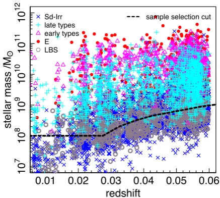
Figure 1. Shown is the redshift – stellar mass distribution for the GAMAn-ear sample. The points are coded according to theHubbletype established in the visual morphology classification. There appears to be no bias towards a particularHubbletype at the higher redshift boundary of our sample.

first instance into bulge- and disc-dominated, little blue spheroid (LBS) and star/artefact. In the following step, the bulge- and disc-dominated objects are further split into single- and multicomponent. Finally, the multicomponent galaxies are sorted into barred and

unbarred. For each galaxy, the result was then translated to aHubble

type: E, S0-Sa, SB0-SBa, Sab-Scd, SBab-SBcd and Sd-Irr, plus the additional LBS, Star and Artefact classifications (see Moffett et al.

2016, for further details). Note that throughout this paper, the terms

early and late type refer to our visual classification of objects being bulge- or disc-dominated and we do not impose any other parameter cuts (e.g. S´ersic index) to classify early or late type.

We perform bulge+ disc decomposition in therband only as

our fitting approach is computationally expensive. For the analy-sis, we do not consider objects classified as stars or artefacts and we excluded one additional galaxy which was too large to be fit robustly. The resulting sample is hereafter called GAMAnear and comprises 7506 galaxies of which 2247 were visually classified as two-component (S0-Sa, SB0-SBa, Sab-Scd, SBab-SBcd) and 5259 as single-component (E, Sd-Irr, LBS) galaxies. Due to the

low-redshift range, this sample extends well below 109_M

allowing

us to study the low-mass end of theM–Re relation. However,

because of the limited volume of our survey, this also means we do not have many very high-mass galaxies to study the curvature

of theM–Rerelation at higher masses. This is important as the

curvature in the (elliptical)M–Rerelation is likely indicative of

the assembly history of the galaxy population (see e.g. Bernardi

et al.2011and references therein).

As shown by Moffett et al. 2016, their fig. 5, the fraction of

galaxy type by mass behave as expected, e.g. the fraction of early-type galaxies increases with increasing mass and the fraction of late-type galaxies decreases. To check whether the sample se-lection in this paper is biased, we show the sample distribution

in the redshift – stellar mass plane in Fig.1. The dashed line shows

the final mass limit used in Section 5 to derive theM–Rerelation.

The figure illustrates the mass segregation of the sample with the early-type galaxies being more massive than the late types. How-ever, there is no clear bias with morphological type or our redshift range, especially at the upper redshift boundary.

at University of St Andrews on October 11, 2016

http://mnras.oxfordjournals.org/

3 B U L G E + D I S C D E C O M P O S I T I O N

Obtaining reliable bulge+disc fits is notoriously difficult,

partic-ularly in an automated fashion for large samples where the signal-to-noise ratio and resolution varies. Typically, 20–30 per cent of au-tomatic fits are, in some way, non-physical. Previous studies have

made use of a logical filter (e.g. Allen et al.2006; see also Simard

et al.2011; Meert et al.2015) to identify unphysical fits (e.g.

com-ponent profiles which cross twice, the switching of the bulge and

disc components etc.; see Allen et al.2006for more details) and

manage these failures by replacement with a single S´ersic fit. As a first step, this reduces the catastrophic failure rate significantly but introduces a bias by removing the subset of two-component systems with poor fits. Following extensive exploration of our data

usingGALFIT3 (Peng et al.2010) embedded inSIGMA(Kelvin et al.

2012), we identify five commonly occurring key factors which lead

to poor and often catastrophic fitting outcomes. These are summa-rized below along with our adopted solution.

(1)Becoming trapped in local minima and/or the limited move-ment of the final converged solution away from the initial conditions.

The Levenberg–Marquart (LM)χ2_{minimization algorithm used by}

GALFIT3 can get stuck in a local rather than the globalχ2minimum, especially when fitting multiple components. One way to overcome this is to vary the initial conditions (i.e. starting points) and repeat the fitting process. Convergence to a common solution, regardless of the starting point, provides confidence that the true minimum has been found. In due course, a full Markov Chain Monte Carlo (MCMC) approach, that appropriately samples the prior distribution should be developed but that is beyond the scope of our current investigation at this stage.

(2)Unphysical solutions, e.g. a scalelength of 0.1 arcsec or a S´ersic index of 20.

In some cases., the bulge or disc fits can migrate to the fit limits im-posed, and these results are often not physical. While it is tempting to reduce the limits to plausible values, this causes a non-physical build-up of the solutions at the limits. Moreover, during the path towards convergence, it can sometimes be seen that solutions mi-grate into extreme values and then back again. To minimize the impact of our boundaries, we imposed no limits on the parameters,

bar the constraint on the centre position, which is set to±5 pixels

to account for the oversampling of the point spread function [PSF, i.e. GAMA pixel size is 0.339 arcsec and SDSS full width at

half-maximum (FWHM)=1.5 arcsec]. Instead, we elect to remove final

solutions which settle on extreme values. We can afford to do this since we have multiple fits for each galaxy, i.e. some starting points lead to extreme outcomes but on the whole most converge to

plau-sible values. Note thatGALFITdoes have some inbuilt constraints,

such as a maximum S´ersic index of 20.

(3)Decision on single or multiple components.

A key problem in galaxy decomposition is to decide how many components are required. Ideally, this should be derivable from the independent 1-, 2- or multicomponent fits. Experimentation with the Akaike and Bayesian Information Criteria (AIC and BIC, respectively) was explored but no obvious automated process for determining the number of components, which agreed with our visual assessments, was identified. This is in part due to the limited information available in single-band fitting. Hence, we adopt our visual classifications as priors, i.e. E, Sd-Irr and LBS galaxies are taken as single-component systems and S0-Sa, SB0-SBa, Sab-Scd and SBab-SBcd as two-component. For completeness, however, we do derive and provide both one- and two-component fits for all systems.

(4)Reversal of the bulge and disc components.

On occasion, the initially assigned bulge component migrates to fit the disc component and the disc to the bulge. This effect was first

noted in Allen et al. (2006) and can be rectified by switching the

components if necessary. Here, regardless of the initial parameters, we assign the component with the lowest half-light radius as the bulge (i.e. inner, more compact component) and the other as the disc (i.e. outer, more extended component). This can, however, lead to cases where the bulge has a lower S´ersic index than the disc (see Appendix A for our treatment of these cases), which, in the majority of cases, is an unphysical solution.

(5)DefaultGALFITerrors do not reflect the full complexity and uncertainty in the final fits.

It is known thatGALFIT(like other fitting codes) often underestimates

the error on the returned parameters (see e.g. H¨aussler et al.2007),

possibly due to the poor treatment of correlated noise in real images. Essentially, the final errors do not provide any indication of fit

confidence. By runningGALFITmultiple times from a grid of initial

conditions, we can assess the level of convergence which can be used to provide more realistic error estimates. This reassessment of the errors is probably the most important outcome of our adoption of a grid of initial conditions, providing some certainty for each galaxy as to the robustness of the fit.

The five strategies above proved critical in reducing the catas-trophic error rate (as assessed from visual inspection) from

∼20 per cent to∼5 per cent enabling us to dispense with the need

for a logical filter, and most importantly obtain realistic errors. We recognize that many of the above could also be addressed by improving the minimization algorithm and implementing an MCMC approach which fully samples the prior distribution. At the present time, however, in the absence of a known prior distribution and limited computing time, we believe our strategies minimize

the obvious systematic issues which arise when using theGALFIT3

engine.

3.1 Construction of a robust decomposition catalogue

3.1.1 The initial grid and convergence

As stated, for completeness, we perform both single and double

(bulge+disc decomposition) component fits in therband on all

7506 galaxies in our sample using one or two S´ersic functions, respectively. We do not constrain any fitting parameters, except for

the inbuilt limits withinGALFIT. Hence, in our two-component fits,

the bulge and disc S´ersic indices are not set to any particular value

(e.g. 1 and 4) as is often done in other studies. We use theSIGMA

(Kelvin et al.2012) wrapper code forGALFIT (Peng et al.2010).

As a front-end wrapper,SIGMA creates cutouts from the GAMA

regions, does a local background subtraction and detects objects and

stars using SEXTRACTOR(Bertin & Arnouts1996). To obtain reliable

S´ersic fits, it is important that local background sky variations are accounted for, yet it is also important to not oversubtract light from the galaxy itself, as this will lead to systematic errors in the galaxy flux measurements. Our local background subtraction is in addition to the background subtraction applied during mosaicking of the GAMA data. The grid size used during this additional sky

estimation depends on the size of the galaxy and varies from 32×32

to 128×128 pixels. Using this variable mesh approach was found

to be the most robust method to remove small-scale sky variations without removing light from the galaxy (for further details, see

Kelvin et al. 2012). After the sky subtraction, SIGMA constructs

at University of St Andrews on October 11, 2016

http://mnras.oxfordjournals.org/

1474

R. Lange et al.

Figure 2. Convergence plot examples for a single-component galaxy in the top panel and a double component galaxy in the bottom panel. The plots show the starting (grey points) and end values (arrow head) for several fit parameters making it easy to evaluate how well the galaxy was fit. For the single-component fits, we show the galaxy’s total magnitude, size and S´ersic index. For the two-component fit, we show the bulge-to-total (B/T) and disc-to-total (D/T) flux ratios of the components instead of the magnitude. The green ellipse is centred at the median output values and its size corresponds to the adopted error on the median. Note that for the single-component fit, the error on the magnitude corresponds to our error floor of 0.11 mag. The dashed lines indicate the fitting outcomes we consider to have failed. Note that the arrow colours correspond to the final S´ersic index values only (if it is grey, then the S´ersic index is outside the range of the values we considered physical, see Section 3.1.4) and each grey point has several arrows associated with it due to the combination of starting values of our initial grid. See the text for a detailed description.

a PSF using PSFEXTRACTOR(Bertin 2013) which is later used to

convolve theGALFITmodels. The SEXTRACTORoutputs are also used

to inform the fitting of neighbouring objects as well as provide

initial starting values for theGALFITrun (for full details onSIGMA, see

Kelvin et al.2012). During the actualGALFITroutine the primary and

all secondary objects are simultaneously modelled using a S´ersic

function. In the case of a two-component fit,GALFITminimizes the

χ2_{over two S´ersic functions centred on the primary object while}

also fitting the secondary objects with a single S´ersic profile. To identify convergence to the global minimum, we use a grid of initial starting points (as previously discussed) for both the bulge and disc components as described below.

(i) Two-component fitting: a total of 88 starting combinations varying input parameters as follows,

(a) ratio of bulge to disc size (bulge size/disc size, RSE=

SEXTRACTORradius):

1:1 (RSE/RSE),

1:2 (0.75×RSE/1.5×RSE),

1:4 (0.5×RSE/2×RSE),

1:9 (0.33×RSE/3×RSE),

(b) two sets of component starting S´ersic index:

n=4+1 (bulge+disc)

n=2.5+0.7 (bulge+disc),

(c) component bulge and disc flux ratio:

60 per cent : 40 per cent (bulge : disc) to 10 per cent : 90 per cent in steps of 5 per cent,

(ii) Single-component fitting: a total of 33 combinations of the input parameters

(a)R=2, 1, 0.5, 0.25×RSE

(b) S´ersic indexn=1, 2, 3, 4

(c) total magnitude mag=1, 0.8×MSE

(d) one additional model starting withR=RSEand mag=MSE

andn=2.5.

RSEandMSEdenote the initial size and magnitude values taken from

the SEXTRACTORoutputs for the entire galaxy.

Fig.2shows an example convergence plot for a single-component

fit (top, G7848) and a double-component fit (bottom, G250228). The

at University of St Andrews on October 11, 2016

http://mnras.oxfordjournals.org/

plots show the grid of initial conditions (grey points) and vectors pointing to the final solution for each parameter combination. We plot the size versus magnitude plane for the single fits and the size versus component light fraction plane for the double fits (bulge component, left, disc component, right). The colour bar at the top shows the S´ersic indices considered and spans the same range for all convergence plots. The arrows pointing to the final output pa-rameters are coloured according to the final S´ersic index. In practice

(e.g. Fig.2, bottom), not all fits converge to a plausible solution and

hence screening is required to remove obvious bad fits. Dashed lines indicate fitting outcomes which were excluded due to bad values

(see the screening descriptions below) or a large reducedχ2_{. If the}

(dashed) lines are grey, the final S´ersic index was outside the range displayed in the colour bar. The green ellipse shows the median so-lution and its size corresponds to the adopted error on the median, i.e. the error is symmetrical and taken to be the average of the 16th and 84th percentile range. We produce convergence plots for all one- and two-component fits of our 7506 galaxies. As mentioned previously convergence towards a tight median value is by no means assured and a number of situations need to be managed, including component flipping, unphysical solutions and poor-quality fits. We refer to this management as screening and define the various steps below.

3.1.2 Screening via profile switching

Each of our 2247 two-component systems will have 88 model out-puts from our grid of initial parameters. When fitting the galaxies, component 1 has been assigned the bulge initial parameters and

component 2 the disc initial values. SinceGALFITcomponents can

migrate significantly, we ensure, after the fitting has finished, that the more compact component is taken as the bulge and the more extended as the disc. However, we find some cases where, even though the bulge is smaller in size, the disc has the higher S´ersic in-dex. Visually inspecting a number of the resulting profiles, we find that the more extreme cases typically are bad fits and flag these (see Appendix A). Additionally, we relax the criterion for switching the components and allow bulges with lower S´ersic index than the disc if they are no more than 10 per cent larger than the disc. For 1447 galaxies, at least one of the 88 parameter combinations required

switching the profiles output byGALFIT.

3.1.3 Screening via rejection of poor-quality fits

We also reject fits with poor reducedχ2_{values. To decide on an}

appropriate reducedχ2_{cut, we randomly inspected 20 fitting}

out-comes for each of 100 two-component galaxies. For each fitting outcome, we decided (by eye) whether it was acceptable or not based on the light profile of the model and the resulting residuals.

Fig.3shows the distribution of reducedχ2_{for these galaxies split}

into ‘good’ and ‘bad’ fitting outcomes, shown as green and red his-tograms, respectively. The vertical dashed line indicates the final

cut of reducedχ2_{=4 which is left deliberately high to ensure that}

even for galaxies with a lot of structure, we exclude none of the acceptable fit outcomes and have enough outputs to evaluate the ‘best’ fit. This cut is also implemented for the single S´ersic fits. In

total, 20 505 (∼10 per cent) of the 197 736 fitting results were

re-moved from the two-component sample and 5686 (∼7 per cent)

from the 173 547 fitting results of the single-component sample.

Figure 3. Shown is the reducedχ2_{distribution of a test sample of 100}

two-component galaxies for which 20 fitting outcomes each were visually inspected. The green histogram shows the fits classified as ‘good’ and the red histogram shows the bad fits. The dashed vertical line is the implemented reducedχ2cut.

3.1.4 Screening via rejection of unphysical fits

Fig.4summarizes the derivedGALFIT-fitted values of all

combina-tions for our bulges and discs showing in the upper panels the bulge (left) and disc (right) sizes, and in the lower panels the bulge (left) and disc (right) S´ersic indices. Taking the top-left panel, we see that the bulge sizes follow two distinctive bands, one at plausible sizes (i.e. 0.1–10 arcsec scales), and one at unphysical sizes (0.001–

0.01 arcsec) given the data resolution of∼1.5 arcsec. We reject the

fitting results which result in overly compact ‘bulges’ and remove these from further considerations (red dashed line). Overly large bulges or discs are not a prominent problem but we remove obvi-ous outliers based on the distribution of all solutions. Similarly, in

Fig.4(bottom), we show the S´ersic index distribution. Once again,

the vertical red dashed lines indicate the division between the fit-ting results we consider physical and those we consider unphysical and that should therefore be rejected. The limits adopted leading to rejection (red dashed lines) are:

(i) for bulge sizes:Re<0.01 arcsec orRe>20 arcsec

(ii) for disc sizes:Re<0.1 arcsec orRe>200 arcsec

(iii) for bulge and disc S´ersic index:n<0.1 orn>15.

These cuts are deliberately permissive and should cut out only the most unrealistic fitting outcomes. For our two-component galaxy sample, of the 197 736 combinations fitted, we reject

17 343 (∼18 per cent) based on bulge size, 616 based on disc size

(<1 per cent), 18 357 (∼19 per cent) based on bulge S´erisc index

and 11 462 (∼12 per cent) based on disc S´ersic index. For the

single-component fits, we reject fitting outcomes based on the same limits as the disc size and S´ersic cuts of the two-component fits. Of the 173 547 combinations fit to the single-component systems, we

re-ject 2753 (∼3 per cent) based on their size and 2355 based on their

S´ersic index (∼3 per cent). In total, 49 688 (∼25 per cent) fitting

results are rejected from our two-component sample fits and 7757

(∼4 per cent) from our single-component fits. Note that, in many

cases, fitting results are rejected by more than one criterion (i.e.

reducedχ2_{and/or size and/or S´ersic index).}

We also screen our galaxies for various flags, described in Ap-pendix A. However, we only consider two flags important during

the componentM–Rerelation fits, namely the very high (or low)

B/T galaxies and reversed S´ersic index galaxies. We deem the high

(and low) B/T galaxies single-component systems and move them

from our two-component sample to our single-component sample.

at University of St Andrews on October 11, 2016

http://mnras.oxfordjournals.org/

1476

R. Lange et al.

Figure 4. The top panel shows the distribution of the output size for all bulges (left) and discs (right) for the fitted two-component models (no re-ducedχ2_{cut has been imposed) of each galaxy (indicated as ‘Number’). The}

dashed vertical lines show the implemented cuts on the size before the me-dian is established. The bottom panel shows the corresponding distribution for the output S´ersic index for the bulges (left) and discs (right). In all panels, the galaxies are sorted byHubbletype with the late-type two-component systems at the top and early-type two-component systems at the bottom. The horizontal dashed black line shows where theHubbletype changes.

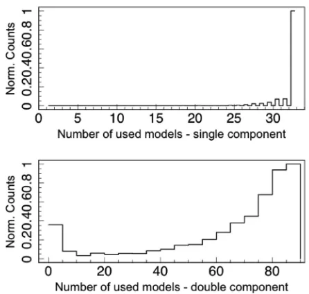
Figure 5. Here we show the distribution of the number of fitting outcomes used to calculate the median. The top panel shows the distribution for single-component fits based on single-single-component galaxies only. The bottom plot shows the distribution of the number of component fits used for two-component galaxies only. It can be seen that the single S´ersic fits generally converge nicely and the two-component fits have a broader distribution with a spike at very low numbers.

Galaxies with inverted S´ersic index have bulges with lowernthan

discs. Visually inspecting several of the profiles, we find that in most

cases, these are bad fits, i.e. we find the disc S´ersic indexn>2. This

itself would not be a problem if the errors reflect our confidence in the fit. Many of these profiles, however, have converged to this unphysical solution. We find 182 late-type two-component systems and 87 early-type two-component systems have inverted S´ersic in-dex and converged profiles. We remove these galaxies from our component consideration, but use their single-component profile

fits to establish their globalM–Rerelation.

3.1.5 Final parameter selection

For each galaxy, we consider two possible profile fit solutions taken from the remaining fitting results:

(i) the minimumχ2_{model with the associated}

GALFITparameters and errors, and

(ii) the median fit values of the remaining fitting results and

the 16th and 84th percentiles (i.e. the 1σ deviation of a normal

distribution) as an uncertainty indicator.

While the minimumχ2_{solution should represent the best formal}

fit from our grid, the median model is our preferred solution, as the errors on the median reflect the level of convergence and robust errors are critical. Note that the median values are calculated for each output parameter individually and do not directly represent any single solution. In cases where the fitting converged, the median and

minimumχ2_{solution will be almost identical and the 16th and 84th}

percentile range often is smaller than theGALFITerrors. We therefore

adopt an error floor of 10 per cent of the median value, which assures that in almost all cases, the median solution is consistent with the

minimumχ2_{solution within the estimated errors.}

Fig.5shows the histogram of the number of the remaining

fit-ting results used to calculate the median for all single-component

at University of St Andrews on October 11, 2016

http://mnras.oxfordjournals.org/

systems (top) and all two-component systems (bottom). The

single-component fits often converge and the histogram peaks at∼33

fitting results with only a small tail towards lower numbers. The two-component fits on the other hand do not converge as often. It

is encouraging that the peak is≥85 fitting results, however, there

is a large fraction of galaxies for which very few solutions remain for the median calculations. In addition, there is a rise towards very low numbers indicating that some galaxies are likely too complex to be fit with two components only. We find that, while the galax-ies with low model counts span the whole mass range, most of them lie close to our upper redshift boundary and were classified as late-type double-component systems. This shows the inherent difficulty of fitting multiple component systems in poorer image quality regimes. In addition to the tightness of the median errors, we can also use the number of fitting results left for the calcula-tion of the median to help establish our confidence in the fitting results.

3.2 Convergence examples

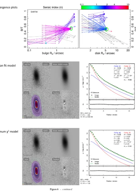
We finish this section by presenting five examples which highlight some of the issues encountered and show that the median values

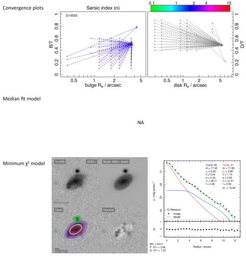
present a robust alternative to the minimumχ2_{solutions. Fig. 6}

(upper panels) shows the convergence plots (as introduced in

Sec-tion 3.1.1 and Fig.2), and diagnostic plots for the median and

minimum-reducedχ2_{solutions (middle and lower panels,}

respec-tively). The four images which make up the diagnostic plots (middle and lower left panels) show, from the top left in a clockwise

direc-tion, the SDSSrband image stamp, the model produced byGALFIT,

the residual and the SEXTRACTOR segmentation map overplotted

on the SDSS image stamp (the primary object is shown in purple

and the secondaries in green). The red and blue ellipse show theRe

of the bulge and disc, respectively. The yellow ellipse is the original SEXTRACTORradius and the cyan ellipses show the radii for which the surface brightness was evaluated. Also shown (middle and lower-right panels) are the 1D light-profile comparisons. The black points are the values extracted from within the blue ellipses, the red and green lines are the 1D light profile for the bulge and disc, evaluated

from theGALFITmodel and the green line is the total light profile.

The lower inset panel shows the residual between the model and data. Below we discuss five examples of various fit and convergence outcomes. We only discuss examples for two-component galaxies here, since we find that the single S´ersic fits generally converge well (e.g. example a):

(i)Example a: full convergence

Fig.6(a) shows the ideal case of full convergence from all

combi-nations of initial parameters. The median and minimumχ2

solu-tion diagnostic plots also show that both reached the same answer. The residual images show little structure and the final errors of the median fit are small as indicated by the green ellipse on the convergence plot. For two-component fits, we consider them fully converged when they have more than 80 fitting results remaining after rejection of spurious fits and the error on the median is set to

the 10 per cent error floor. This is the case for 423 (∼19 per cent)

galaxies. Similarly, for single components, over 30 fitting results must remain for the median calculation and all errors are set to the

10 per cent error floor. This is true for 4566 (∼87 per cent)

single-component galaxies.

(ii)Example b: partial convergence

The median and minimum-reducedχ2_{model diagnostic plots in}

Fig.6(b) show good agreement. From the convergence plot, it is

obvious that many of the solutions found byGALFITwere rejected

during the screening process, due to an unphysical S´ersic index

or high reducedχ2_{. The remaining models after screening show}

convergence resulting in a good solution with tight errors. For two-component systems, we consider good convergence to be reached when we have 60–80 solutions remaining, with the errors set to the

10 per cent error floor. This is the case for 297 (∼13 per cent)

galax-ies. Equivalently, for single components, 25–30 solutions must re-main for the median calculation with the errors set to the error floor.

We find this true for 220 (∼4 per cent) single-component galaxies.

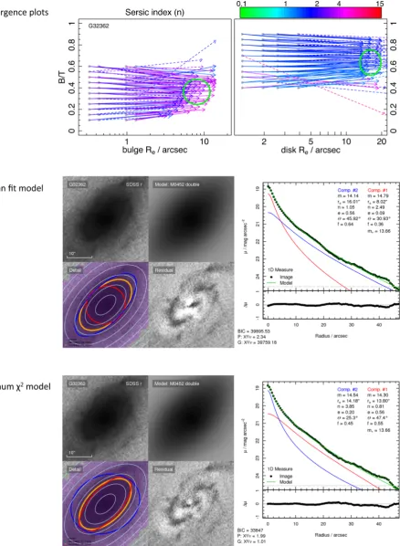
(iii)Example c: two plausible solutions

The diagnostic plots in Fig. 6(c) suggest that the median model

gives a physically more meaningful two-component solution than

the minimum-reducedχ2_{solution which is converging towards a}

single-component solution. The convergence plot, however, high-lights that the median solution is not one of the actual solutions

found byGALFIT. Nevertheless, the errors on the median (green

er-ror ellipse) enclose both solutions. While the median fit cannot be considered as robust, this uncertainty is fairly reflected in the final errors. To establish whether several plausible solutions have been found, we test how many solutions are near the median. If less than 10 per cent of the solutions of the median, for at least one of

the size, S´ersic index or B/T values of either the bulge or disc,

lie within 10 per cent (i.e. the error floor), then we consider the fits to have converged to several plausible solutions which are distinct

from the median. This is the case for 205 (∼5 per cent)

double-component systems. For the single-double-component systems, we

con-sider the size, S´ersic index and magnitude and find six (<1 per cent)

single-component galaxies have converged to several distinct solutions.

(iv)Example d: no convergence

Fig.6(d) shows a case where no obvious single converged

solu-tion is found, but the median model returns acceptable parameters with an appropriately broad error distribution. The diagnostic plots also show that the median model returns a physically possible

so-lution with good residuals. The minimum χ2 _{solution, however,}

returns a fit where the bulge, even though it has a smaller Re is

the dominant component in the outer parts of the galaxy. Since the errors associated with the median model are large, this

partic-ular galaxy will not have much influence on theM–Re relation

we fit in Section 5.2, but using the median parameters and large error bars means that the galaxy will not be discarded from the sample. To test non-convergence, we use the same metric as in ex-ample 3, i.e. the percentage of solutions found within 10 per cent of the median. We consider galaxies not clearly converged if more than 10 per cent but less than 50 per cent of the solutions lie close

to the median. We test the size, S´ersic index and B/T

measure-ments for the bulge and disc and find for 931 (∼41 per cent)

two-component systems that at least one of them is not converged. For

the single-component systems, this is the case for 141 (∼3 per cent)

galaxies.

(v)Example e: no solution

Fig.6(e) shows a case where convergence is found, however, all fits

are excluded from the final catalogue due to the screening process. No median model diagnostic plot is shown due to all fit parameters

being unrealistic. Only 120 (∼5 per cent) of our two-component

galaxies and 129 (∼2.5 per cent) of our single-component systems

fall into this category.

Convergence plots for all systems are available from the GAMA data base.

at University of St Andrews on October 11, 2016

http://mnras.oxfordjournals.org/

1478

R. Lange et al.

Figure 6. Presented are the convergence plots (top) and corresponding diagnostic fit plots for the median fit model (middle) and minimum-reducedχ2_solution

(bottom). We show four examples ranging from full convergence to no convergence (panels a, b, c, d) and one example where all fits are unrealistic (panel e). A detailed discussion can be found in the text.

at University of St Andrews on October 11, 2016

http://mnras.oxfordjournals.org/

Figure 6 – continued

at University of St Andrews on October 11, 2016

http://mnras.oxfordjournals.org/

1480

R. Lange et al.

Figure 6 – continued

at University of St Andrews on October 11, 2016

http://mnras.oxfordjournals.org/

Figure 6 – continued

at University of St Andrews on October 11, 2016

http://mnras.oxfordjournals.org/

1482

R. Lange et al.

Figure 6 – continued

4 C O M P O N E N T M A S S E S

To derive the M–Re relations for our galaxy components, we

now need component mass estimates. For the single S´ersic fits, we can directly use the GAMA stellar mass estimates from the StellarMassesv18 catalogue and apply the flux-scale correction

(for a detailed description, see Taylor et al.2011, essentially the

flux-scale correction accounts for the differences between aperture matched and S´ersic photometry). These masses are based on syn-thetic stellar population models from the BC03 library (Bruzual &

Charlot2003) with a Chabrier (2003) initial mass function and the

Calzetti et al. (2000) dust obscuration law. We find that, for our

sample, the typical error, which has been derived in a Bayesian

way (sections 3.2–3.4 of Taylor et al. 2011), is of the order of

∼0.12 dex.

For the double-component galaxies, we calculate the component

mass from the component colours (Driver et al.2006) using the

relationship between optical colour (g−i) and mass-to-light ratio

as calibrated by Taylor et al. (2011):

logM_∗/M _{= −}0.68+0.7(g−i)−0.4(Mi−4.58), (1)

whereMiis the absolute magnitude in theiband and we use the

(g−i) colour of either the bulge or disc to calculate the

com-ponent mass. The stellar masses derived via equation (1) are estimated to be accurate within a factor of 2. Note that this

at University of St Andrews on October 11, 2016

http://mnras.oxfordjournals.org/

equation is sensitive to the evolution of colour and magnitude, how-ever, as our sample has a low-redshift range, the effects will be negligible.

Ideally, we would use bulge and disc colours derived from the

bulge+disc decompositions in the gandiband, however, this

is beyond the scope of this paper. Hence, we have to estimate the colours of the components. For this, we measure the PSF and total

magnitudes of our galaxies in theg, r,andiband and we then use the

GALFITmeasuredrband component magnitudes and B/T to estimate the bulge and disc colours.

We measure the core (i.e. PSF) and total magnitudes, which

we correct for foreground extinction, in theg, r,andiband using

LAMBDAR, a code developed to measure PSF+weighted aperture

pho-tometry (for more details, see Wright et al.2016). We then equate the

colours measured using the PSF magnitudes to bulge colour mea-surements (i.e. assuming the bulge has no colour gradient) and

com-bine these colours with ourrband bulge magnitude fromGALFITto

obtain bulge flux measurements in bothgandi(i.e.mi,bulge=mr,bulge

−(r−i)PSF,bulge). In cases where the bulge colours could not be measured, we use the median bulge colour of the entire population as there is no significant trend between bulge colour and mass. We

derivegandidisc fluxes by assuming that the disc flux in each band

is equal to theLAMBDARtotal flux minus the previously derived bulge

flux.

We examine the disc (g−i) colour distribution and find a small

number of extreme outliers (>3σ) from the colour distribution,

whose disc (g−i) colours we subsequently replace with the running

median disc (g−i) colour.

Finally, we use the derived bulge and disc (g−i) colours and

totaliband magnitudes to derive stellar mass estimates for each

component according to equation (1). The component colour versus

S´ersic index distribution is shown in Fig.7for bulges (top) and

discs (bottom). Fig.7shows that for late-type galaxies, bulges are

generally redder than discs but for early-type galaxies, the colours are very similar (for a detailed study of the wavelength dependence

of bulge+disc decompositions in GAMA, see Kennedy et al.2016).

But it also highlights the problem galaxies for which the component colour had to be set to the median colour (vertical band in the bulge plot, top) in order to be able to calculate a stellar mass estimate.

5 M–Re R E L AT I O N S

We now present theM–Rerelations, first, for the differentHubble

types and secondly, by structural components. We conclude our

analysis by presenting a combinedM–Re relation for disc (i.e.

Sd-Irr galaxies and disc components) as well as spheroids (i.e. ellipticals and classical bulge components).

Fig. 8shows the selection of the final sample, based on total

stellar mass and single S´ersic profile fits, used to fit theM–Re

relation. Note that we do not consider any galaxies below M_∗=

108_M

, since number counts are too low to establish a robust

weight (after flux-scale correction, this reduces the sample to 6788 galaxies). First, we find and exclude outliers from the general mass–

size distribution (top panel of Fig.8). For this, we fit the entire

sample with a simple power law and remove all galaxies which

are more than 3σ sigma offset from the best-fitting linear relation

(28 galaxies in total). We then establish the lower mass limit for a

volume-limited sample atz=0.06. In the middle panel of Fig.8,

we plot the maximum redshift at which each galaxy can be seen versus its stellar mass. To establish the lower mass limit of a volume-limited sample, we find the point at which more than 95 per cent of

00 .2 0 .4 0 .6 0 .8 1 −

1 0 1 2 3

Norm. Counts

−1 0 1 2 3

0.1 1 10 bulge (g-i) bulge n S0-Sa SB0-SBa Sab-Scd SBab-SBcd

0 0.20.40.60.8 1

0.1 1 10 Norm. Counts 0 0 .2 0.4 0 .6 0.8

1 −1 0 1 2 3

Norm. Counts

−1 0 1 2 3

0.1

1

10

disk (g-i)

disk n

0.2 0.4 0.6 0.8 1

0.1

1

10

Norm. Counts

Figure 7. Shown are the (g−i) colour versus S´ersic index distributions for the bulges (top) and discs (bottom) in our two-component galaxy sample. The colour coding in both plots is the same with late types in blue and early types in magenta. The bulges of late-type galaxies have smaller S´ersic indices than the early-type bulges. The S´ersic index distribution of the late-type discs also peaks slightly lower than the early-late-type discs. Late-late-type discs are also bluer than early-type discs.

our galaxies could be seen at a redshift of 0.06 (i.e. their maximum

redshift is zmax≥ 0.06, indicated as the dashed line). We find a

lower mass limit ofM∗=109_M

(solid blue line), which would

reduce our sample size to 3679 galaxies. To include lower mass galaxies, we implement a smooth volume- and mass-limited sample

for galaxies below M_∗=109_M

. For each galaxy, we evaluate

if their measured redshift is larger than their expected maximum redshift and remove them (1624 galaxies removed). The bottom

panel of Fig.8shows the resulting sample distribution. All galaxies

in red are included in our final sample (5136 total) and all grey points are excluded from the volume-limited sample. For all galaxies below

at University of St Andrews on October 11, 2016

http://mnras.oxfordjournals.org/

1484

R. Lange et al.

stellar mass /Mʘ

Re

/kpc

108 109 1010 1011 1012

0.1

1

10

100 GAMA II (0.002<z<0.06) best fit

3 sigma

stellar mass /Mʘ

maximum redshift

108 109 1010 1011 1012

0 0 .1 0.2 0 .3 0.4 0 .5

z limit: 0.06 mass limit: 9.0

stellar mass /Mʘ

redshift

108 109 1010 1011 1012

0.01

0.03

0.05

Figure 8. The top panel shows the total stellar mass – half-light size dis-tribution (derived from single S´ersic fits) of the GAMAnear sample. All galaxies more than 3σoffset from the line of best fit are removed as outliers from ourM–Rerelation fits. The middle panel shows the total stellar mass

– maximum redshift distribution of the sample. The blue dashed line shows our redshift limit and the solid blue line the lower mass limit for a volume-limited sample. All galaxies to the right of the mass limit and above the redshift limit are included in the volume-limited sample. The bottom panel shows the total stellar mass – redshift distribution of our sample. For all galaxies below 109_M

, we have implemented a smooth volume-limited sample selection. Our final sample is highlighted in red.

M∗=109M, we also calculate a V/Vmaxweighting based on

their redshift and our sample redshift limits of 0.002< z <0.06.

For galaxies with M_∗>109_M

, the V/Vmaxis set to 1. To ensure

that we only include galaxies with good, physical fits, we require:

(i) the flux-scale correction is within 0.5 and 1.5;

(ii) the components have S´ersic indices within the range 0.3<n

<10;

(iii) the components are resolved, i.e.Re>0.5×FWHM of the

PSF which is determined from each galaxy’s fit image individually;

(iv) at least five solutions remained to calculate the median fit parameters.

This reduces the sample size to 2669 single-component and 1470 double-component systems.

We adopt a simple power law, following Shen et al. (2003) and

Lange et al. (2015), to fit theM–Rerelation:

Re=a

M∗

1010_M

b

, (2)

whereRe is the effective half-light radius in kpc and M_∗is the

mass of the galaxy. To perform the actual fitting, we utilize the HYPERFITpackage (Robotham & Obreschkow2015) which estimates

theM–Rerelation via Bayesian inference for each morphological

group and component. During fitting, we assume uniform priors

and each galaxy is weighted by its V/Vmaxand the (convergence)

errors for each individual galaxy are fully taken into account during the fitting process.

5.1 GlobalM–Rerelations byHubbletype

To establish the global (i.e. single-component S´ersic fit)M–Re

relation byHubbletype, we have grouped the GAMAnear sample

into five populations:

(i) 1564 late-type single-component galaxies (including 40

high/low B/T galaxies),

(ii) 890 late-type multicomponent systems (comprised of Sab-Scd and SBab-SBcd galaxies) of which 708 have also good two-component fits,

(iii) 580 early-type multicomponent systems (which include S0-Sa and SB0-SBa galaxies) of which 493 have also good two-component fits,

(iv) 806 early-type single-component (including 33 high B/T

galaxies), and (v) 372 LBS.

The resulting globalM–Rerelations are shown in panel (i) of

Fig.9, from left to right, the plots are (a) Sd-Irr, (b) visually late-type

multicomponent systems, (c) visually early-type multicomponent systems, (d) ellipticals and (e) LBS. The fit parameters can be

found in Table1(i).

We find that the single S´ersicM–Rerelation fits to the different

morphological types lie on almost parallel lines (i.e. comparable gradients but offset in normalization). Most two-component systems are more massive than Sd-Irr galaxies, but compared at the same mass, we find that two-component systems are smaller than Sd-Irr galaxies. Compared to the ellipticals, however, we find that two-component systems are larger at a given mass. This corroborates the composite nature of these galaxies, i.e. the disc surrounding the

bulge makes their globalReappear larger than ellipticals but smaller

than Irr galaxies at a given mass, with the offset between the Sd-Irr and elliptical relation depending on the relative dominance of the disc or bulge component. The LBS galaxies, on the other hand, are

our smallest and least massive population. The slope of theirM–Re

relation is flatter than that of any of the other morphological types. Nevertheless, their sizes are mostly consistent with an extension of the elliptical population. In fact, within the errors, the LBS relation is

consistent with the low-mass elliptical relation (M∗<1010_M

),

see Table1(ii).

Here our morphological subdivisions are finer than in our previ-ous work (L15) but broadly agree. In detail, our Sd-Irr class has a

steeperM–Rerelation than the late-type relation in L15. This is

at University of St Andrews on October 11, 2016

http://mnras.oxfordjournals.org/

Figure 9. The top panel (i) shows the globalM–Rerelation for: (a) Sd-Irr (blue), (b) late-type multicomponent (dark purple), (c) early-type multicomponent

(rose), (d) ellipticals (red), and (e) LBS (grey) galaxies. Panel (ii) shows, from left to right, the componentM–Rerelation for late-type discs (cyan) and

bulges (purple), plots (f) and (g), respectively. We also plot the global S(B)ab–S(B)cd relation from panel (b) in comparison. The early-type discs (magenta) and bulges (dark red) are shown in plots (h) and (i). Again we plot the global S(B)0–S(B)a (shown in panel c) in comparison. The grey shaded areas indicate where our smooth volume-limited sample selection starts and galaxies are upweighted by their V/Vmax. The black lines are the 90th, 68th and 50th percentiles

of the respective mass–size distributions. The arrows show from which population the components were derived. Finally, we show all globalM–Rerelations

in comparison in the far right plot in panel (ii). This highlights the similarities between the different populations, i.e. the relations are parallel but offset from each other depending on their bulge fraction.

Table 1. The regression fit parameters to equation (2) for the different

Hubbletypes and structural components as well as a combined early- and

late-type relation (see Fig.9).

Case a/kpc b

(i)Hubbletype

Sd-Irr 6.347±0.174 0.327±0.008

S(B)ab-S(B)cd 5.285±0.098 0.333±0.009

S(B)0-S(B)a 2.574±0.051 0.326±0.015

E 2.114±0.035 0.329±0.01

LBS 2.366±0.166 0.289±0.019

(ii) Additional mass constraints E (M_∗≥1010_M

) 1.382±0.065 0.643±0.032

E (M_∗≥2×1010_M

) 0.999±0.089 0.786±0.048

E (M_∗<1010_M

) 1.978±0.077 0.265±0.022

E (M_∗<2×1010_M

) 2.108±0.041 0.326±0.012

(iii) Structural components

late-type disc 6.939±0.17 0.245±0.008

late-type bulge 4.041±0.129 0.339±0.014

early-type disc 4.55±0.097 0.247±0.015

early-type bulge 1.836±0.054 0.267±0.026 (iv) Combined case

all discs 5.56±0.075 0.274±0.004

all discs+LTB 5.125±0.065 0.263±0.004 finalz=0 discs 5.141±0.063 0.274±0.004

E+ETB 2.033±0.028 0.318±0.009

finalz=0 spheroids 2.063±0.029 0.263±0.005 global late types 4.104±0.044 0.208±0.004

Table 2. Fitting parameters taken from L15 (Table2,3and B2) for the rband morphological late- and early-typeM–Rerelation.

Case a b

Late type 3.971±1.745 0.204±0.018

Early type 1.819±1.186 0.46±0.023

Early typeM_∗>2×1010_M

1.390±1.557 0.624±0.033

an effect of our sample selection. In fact, fitting anM–Rerelation

to a combined sample of Sd-Irr and all two-component systems [see

Table1(iv)] results in a relation fully consistent with the late-type

relation in L15 (reproduced in Table2). Our elliptical class has a

shallowerM–Re relation compared to the early-type relation in

L15. This is also largely a sample selection effect, caused by the relative increase in the number of low-mass to high-mass ellipti-cals within the sample. Fitting a high-mass elliptical relation (see

Table1(ii), similar to L15, with M∗>1010_M

), we again find

good agreement with our earlier work.

5.2 M

–

The distributions and fits to the structural componentM–Re

rela-tions are shown in panel (ii) of Fig.9and the fitting parameters can

be found in Table1(iii).

From left to right, panel (ii) shows the late-type discs and bulges (LTD and LTB, plots f and g, respectively) followed by early-type discs and bulges (ETD and ETB, plots h and i). In each panel, we also

show the globalM–Rerelation of the population they were derived

from, which is indicated by the large black arrows. Not surprisingly, we find that generally discs are larger and bulges are smaller than the global single S´ersic fits of the population they were derived from.

Additionally, our data show that the componentM–Rerelations

at University of St Andrews on October 11, 2016

http://mnras.oxfordjournals.org/

1486

R. Lange et al.

Figure 10. Shown are the relative fractional deviations of the different components from the best-fittingM–Rerelation of the tested parent population. The

left-hand plot shows the deviation of the data from the Sd-IrrM–Rerelation and the right-hand plot shows the deviation from the elliptical relation. In both

plots, the area under the curve has been normalized over the range of deviations shown in the plot.

are typically less curved than the global relation they were derived from. However, the late-type discs are an exception to this and show a slight upward curvature at high masses. This is in qualitative

agreement with results from Bernardi et al. (2014) who found that

the discs of late-type galaxies cannot be fit with a single power law, whereas the bulges of early-type galaxies follow a pure power law which is not exhibited by their parent population.

We now wish to establish whether these component fits are

con-sistent with the Sd-Irr or EM–Rerelations. In particular, we wish

to test the following hypotheses:

(a) ETD and Sd-Irr galaxies are associated, (b) ETB and ellipticals are associated, (c) LTD and Sd-Irr galaxies are associated, (d) LTB and ellipticals are associated, (e) LTB and Sd-Irr galaxies are associated, (f) LBS and ellipticals are associated, (g) LBS and Sd-Irr galaxies are associated,

(h) S(B)ab–S(B)cd systems fit with a single component (see Sec-tion 5.3) and Sd-Irr galaxies are associated.

In Fig.10, we visualize the affiliation of various components with

either the Sd-Irr (left) or ellipticals (right) by plotting their relative deviations, defined as

(Robserved−Rpredicted)/Rpredicted, (3)

whereRobserved represents the sizes of the tested populations, and

Rpredicted represents the predicted size using either the Sd-Irr or

ellipticalM–Rerelation. In both panels, the area under the curve

has been normalized and each population is colour coded as shown in the legend with the dashed, vertical black line showing the peak of the deviations for the Sd-Irr galaxies and ellipticals, i.e. the populations to which we compare. The disc components, late-type bulges and the global late-type populations all broadly align with the Sd-Irr relation. The late-type discs tend to higher deviations indicating that they are larger than the Sd-Irr population, however,

their peak deviation is close to 0. The good agreement of the late-type bulges with the Sd-Irr relation hints at their possible ‘pseudo’-bulge nature which is corroborated by their S´ersic index distribution. On the other hand, dust in latet-type galaxies can artificially lower the S´ersic index of LTB, making them appear larger and thus fall within the parameter space of the Sd-Irr relation. Ellipticals, early-type bulges and LBS on the other hand do not align with the Sd-Irr relation and their distributions are completely offset. Conversely, we find that the LBS and early-type bulges visually align with

the ellipticalM–Re relation. They have similar peaks, however,

the early-type bulges have a broader distribution, which is in good

agreement with the larger scatter observed in Fig.9. Whether this

is intrinsic or a by-product of the decomposition is unclear. Late-type bulges, discs and Sd-Irr galaxies are offset from the elliptical distribution and do not follow their relation.

In addition to the qualitative nature of Fig.10, we also perform a

two sample Kolmogorov–Smirnoff-test (KS-test) for each

hypoth-esis. For this, we compare the different samples to the M–Re

relation of either Sd-Irr or elliptical galaxies. Since the KS-test, in essence, compares the cumulative distributions of two populations in one dimension, it does not take into account the spread of our

data around theM–Rerelation. Hence, we decided to bin our data

inlog (M)=0.2 steps to establish the median mass and size of

the bin and we use the median bin mass to calculate the expected

size based on either the Sd-Irr or ellipticalM–Re relation. This

also allows us to test whether the expected size distribution from

theM–Re relation fit agrees with the observed median size

dis-tribution of the sample, even for cases which have only little or no overlap in the mass–size plane (e.g. LBS galaxies and the elliptical

M–Rerelation). The resulting KS statistics are shown in Table3.

For our tested assumptions, combining the results of Fig.10and the

KS-test, we conclude:

(i) a,b,c,e,f,h=True,

(ii) d,g=False.

at University of St Andrews on October 11, 2016

http://mnras.oxfordjournals.org/